Enhancing Geophysical Modeling with Bayesian Hierarchical Techniques

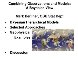
1. Combining Observations and Models: A Bayesian ViewMark Berliner, OSU Stat Dept • Bayesian Hierarchical Models • Selected Approaches • Geophysical Examples • Discussion

2. Main Themes Goal: Develop probability distributions for unknowns of interest by combining information sources: Observations, theory, computer model output, past experience, etc. Approaches: Bayesian Hierarchical Models Incorporate various information sources by modeling priors data model or likelihoods

3. Bayesian Hierarchical Models • Skeleton: • Data Model: [ Y | X , q ] • Process Model Prior: [ X | q ] • Prior on parameters: [ q ] • Bayes’ Theorem: posterior distribution: [ X , q | Y] • Compare to “Statistics”: [ Y | q ] [ q ] “Physics”: [ X | q (Y) ]

4. Approaches • Stochastic models incorporating science • Physical-statistical modeling (Berliner 2003 JGR) From ``F=ma'' to [ X | q ] • Qualitative use of theory (eg., Pacific SST model; Berliner et al. 2000 J. Climate) • Incorporating large-scale computer models • From model output to priors [ q ] • Model output as samples from process model prior [ X | q ] almost ! • Model output as ``observations'' (Y) • Combinations

5. Glacial Dynamics (Berliner et al. 2008 J. Glaciol) Steady Flow of Glaciers and Ice Sheets • Flow: gravity moderated by drag (base & sides) & ….stuff…. • Simple models: flow from geometry Data: Program for Arctic Climate Regional Assessments & Radarsat Antarctic Mapping Project • surface topography (laser altimetry) • basal topography (radar altimetry) • velocity data (interferometry)

8. Modeling: surface – s, thickness – H, velocity - u Physical Model • Basal Stress: t = - rgH ds/dx (+ “stuff”) • Velocities: u = ub + b0 H tn where ub = k tp+ ( rgH )-q Our Model • Basal Stress: t = - rgH ds/dx + h where h is a ``corrector process;” H, s unknown • Velocities: u = ub + b H t n + e where ub = k t p+ ( rgH )-q or a constant; b is unknown, e is a noise process

10. Wavelet Smoothing of Base

11. Results: Velocity

12. Results: Stress and Corrector

13. Paleoclimate (Brynjarsdóttir & Berliner 2009) Climate proxies: Tree rings, ice cores, corals, pollen, underground rock provide indirect information on climate • Inverse problem: proxy f(climate) Boreholes: Earth stores info on surface temp’s • Model: Heat equation Borehole data f(surface temp’s) • Infer boundary condition (initial cond. is nuisance)

15. Modeling Y r h • Data Model: Y | Tr, q ~ N( Tr + T0 1 + q R(k), s2I) true temp Adjustments for rock types, etc. • Process Model: heat equation applied to Tr with b.cond. surface temp history Th Tr | Th ,q ~ N( BTh , s2I) Th | q ~ N( 0 , s2I)

19. In progress: • Combining boreholes (parameters and b.cond as samples from a distribution) • Combining with other sources and proxies

22. Bayesian Hierarchical Models to Augment the Mediterranean Forecast System (MFS)‏ Ralph Milliff CoRA‏ Chris Wikle Univ. Missouri Mark Berliner Ohio State Univ. . Nadia Pinardi INGV (I'Istituto Nazionale di Geofisica e Vulcanologia) Univ. Bologna (MFS Director)‏ Alessandro Bonazzi, Srdjan Dobricic INGV, Univ. Bologna

23. Bayesian Modeling in Support of Massive Forecast Models • MFS is an Ocean Model • A Boundary Condition/Forcing: Surface Winds • Approach: produce surface vector winds (SVW), for ensemble data assimilation • Exploit abundant, “good” satellite wind data (QuikSCAT) • Samples from our winds-posterior ensemble for MFS (Before us: coarse wind field (ECMWF))

24. “Rayleigh Friction Model” for winds (Linear Planetary Boundary Layer Equations) (neglect second order time derivative) discretize: Theory Our model

25. 10 members selected from the Posterior Distribution (blue)‏ BHM Ensemble Winds 10 m/s

26. Approaches • Stochastic models incorporating science • Physical-statistical modeling (Berliner 2003 JGR) From ``F=ma'' to [ X | q ] • Qualitative use of theory (eg., Pacific SST model; Berliner et al. 2000 J. Climate) • Incorporating large-scale computer models • From model output to priors [ q ] • Model output as samples from process model prior [ X | q ] almost ! • Model output as ``observations'' (Y) • Combinations

27. Part B) Information from Models • Develop prior from model output • Think of model output runs O1, … , On as samples from some distribution • Do data analysis on O’s to estimate distribution • Use result (perhaps with modifications) as a prior for X • Example: O’s are spatial fields: estimate spatial covariance function of X based on O’s. • Example: Berliner et al (2003) J. Climate

28. Model output as realizations of prior “trends” • Process Model PriorX = O + hq where h is “model error”, “bias”, “offset” • [ Y | X , q ] is measurement error model: Y = X + eq • Substitution yields [ Y | O , hq , q ] Y = O + hq + eq • Modeling his crucial (I have seen h set to 0)

29. Model output as “observations” • Data Model:[ Y, O | X , q ] ( = [ Y | X, q ] [ O | X , q]) • [ O | X , q ]to include “bias, offset, ..” • Previous approach: start by constructing [ X | O , q ] This approach: construct [ O | X , q] • Model for “bias” a challenge in both cases • This is not uncommon, though not always made clear

30. A Bayesian Approach to Multi-model Analysis and Climate Projection (Berliner and Kim 2008, J Climate) Climate Projection: • Future climate depends on future, but unknown, inputs. • IPCC: construct plausible future inputs, “SRES Scenarios” (CO2 etc.) • Assume a scenario and get corresponding projection

31. Hemispheric Monthly Surface Temperatures • Observations (Y) for 1882-2001. Data Model: Gaussian with mean = true temp. & unknown variance (with a change-point) • Two models (O): PCM (n=4), CCSM (n=1) for 2002-2197, and 3 SRES scenarios (B1,A1B,A2). Data Model: assumes O’s are Gaussian with mean = bt + model biast (different for the two models) and unknown, time-varying variances (different for the two models) • All are assumed conditionally independent

32. Notes (Freeze time) • Data model for kth ensemble member from Model j: Ojk = b + bj + ejk • b is common to both Models • bj is Model j bias • E( ejk ) = 0 and variances of e’s depend on j • Computer model model: b = X + e where E(e) = 0 • Priors for biases, variances, and X • Extensions to different model classes (more b’s) and richer models are feasible.

34. IPCC (global) Us (NH)

36. Discussion: Which approach is best? • Depends on form and quality of observations and models and practicality • Develop prior for X from scientific model (part A)offers strong incorporation of theory, but practical limits on richness of [ X | q ] may arise • Model output as “observations” • Combining models: Just like different measuring devices; • Nice for analysis & mixed (obs’ & comp.) design • Need a prior [ X| q ] • Model output as realizations of prior “trends” • Most common among Bayesian statisticians • Combining models: like combining experts

37. Discussion: Models versus Reality Need for modeling differences between X’s and O’s. Model “assessment” (“validation”, “verification”) helps, but is difficult in complicated settings: • Global climate models. Virtually no observations at the scales of the models. • Tuning. Modify model based on observations. • Observations are imperfect, and are often output of other physical models. • Massive data. Comparing space-time fields

38. Discussion, Cont’d • Part C) Combining approaches • Example: Wikle et al 2001, JASA. Combined observations and large-scale model output as data with a prior based on some physics • Usually, many physical models. No best one, so it’s nice to be flexible in incorporating their information Thank You!