CAPM and APT
CAPM and APT. Chapter 15. Background. Chapter extends concepts developed in Chapter 14 concerning Asset weights Portfolio expected return Portfolio variance-covariance formula Asset allocation line. Investment Opportunities in Risk-Return Space. Markowitz Efficient Portfolios.

CAPM and APT
E N D
Presentation Transcript
CAPM and APT Chapter 15 Chapter 15: CAPM and APT
Background • Chapter extends concepts developed in Chapter 14 concerning • Asset weights • Portfolio expected return • Portfolio variance-covariance formula • Asset allocation line Chapter 15: CAPM and APT
Investment Opportunities in Risk-Return Space Markowitz Efficient Portfolios Individual assets contain both diversifiable and non-diversifiable risk and are not efficient investments. Efficient Frontier—these portfolios contain only undiversifiable risk Individual assets Chapter 15: CAPM and APT
Borrowing and Lending at the Risk-Free Rate • If we add borrowing and lending at the risk-free rate to Figure 14-4 the investment opportunities can be extended • A riskless asset must have a variance of zero, by definition • The efficient frontier curve is now dominated by the capital market line Chapter 15: CAPM and APT
Borrowing and Lending at the Risk-Free Rate Chapter 15: CAPM and APT
The Capital Market Line • The formal equation for the capital market line is: Chapter 15: CAPM and APT
The Market Portfolio • Portfolio M is known as the market portfolio • Equilibrium portfolio containing all the assets in the world in the proportions they are supplied • Represents the single portfolio all rational investors want to own • Because it can be used to create the dominant CML • A useful theoretical concept • Return that security market indexes approximate Chapter 15: CAPM and APT
The Separation Theorem • All investors desiring Markowitz diversification will select Portfolio M • The next question is: • How should the investment in Portfolio M be financed? • Highly risk-averse investors will select a lending portfolio • Aggressive investors will select a leveraged (borrowing) portfolio Chapter 15: CAPM and APT
The Separation Theorem • The decision to invest in portfolio M is separate from the decision as to whether the investor will be a borrower or a lender Chapter 15: CAPM and APT
Assumptions Underlying Portfolio Theory • Four assumptions underlie all portfolio theories based on the efficient frontier • Rate of return is the most important investment outcome • Investor’s risk estimates are proportional to the standard deviation or variance they perceive • Investors are willing to base their decisions on only the expected return and variance (or standard deviation) of the expected return • For any risk class, investors desire a higher rate of return to a lower one Chapter 15: CAPM and APT
Assumptions Underlying the CML, SML and CAPM • Any amount of money can be borrowed or lent at the risk-free rate of interest • All investors visualize the same expected return, risk and correlation for any specified asset (homogeneous expectations) • All investors have a one-period investment horizon • All investments are infinitely divisible • No taxes or transaction costs exist • No inflation or changes in interest rates exist • Capital markets are a static equilibrium (supply equals demand) • The market portfolio contains all assets in the proportions in which they exist Chapter 15: CAPM and APT
Assumptions Underlying the CML, SML and CAPM • Assumptions are unrealistic • But provide a concrete foundation • Final test should be the theory’s predictive power, not the realism of its assumptions Chapter 15: CAPM and APT
Rationale for the SML • Economic rationale based on the manner in which the assets in a diversified portfolio covary • Markowitz portfolio analysis • Find securities with low covariances with the market • Reduce portfolio risk • Since investors will prefer securities with low covariances, securities with high (low) covariances will fall (rise) in price Chapter 15: CAPM and APT
Security Market Line • Equation of the SML Represents the risk-adjusted rate to be used when finding the present value of an asset (when considering systematic risk). Chapter 15: CAPM and APT
Security Market Line In equilibrium every asset should be priced as a linear function of its covariance with the market. Chapter 15: CAPM and APT
SML vs. CML • Individual securities will lie on the SML if they are correctly priced • But individual securities will lie below the CML • They have a high amount of diversifiable risk • Efficient portfolios will lie on the CML • The SML does not consider diversifiable risk • Can be eliminated via simple diversification Chapter 15: CAPM and APT
Restating the SML • The beta regression slope coefficient is an index of an asset’s undiversifiable or systematic risk • An asset’s covariance of returns with the market is also a measure of undiversifiable risk • Two measures are mathematically equivalent Chapter 15: CAPM and APT
Restating the SML • SML may be equivalently restated using the beta coefficient • The restated SML: Chapter 15: CAPM and APT
Over- and Under-Priced Assets • Point U (Slide 15) is an underpriced asset • Has an abnormally high return for its systematic risk • Will experience high demand and a subsequent increase in price until return equates to U • Point O (Slide 15) is an overpriced asset • Has an abnormally low return for its systematic risk • Price will fall due to lack of demand • Assets on the SML are in equilibrium and will remain so until • Systematic risk changes, the risk-free rate changes, etc. Chapter 15: CAPM and APT
Negative Correlation with the Market Portfolio • Point N (Slide 15) is a security with a negative covariance (beta) with the market • The equilibrium rate of return is below the risk-free rate • Gold mining stocks may have negative betas Chapter 15: CAPM and APT
Discontinuity Between Expected Value Theory and Historical Data • Expected returns are determined by expected risk • Investors do not use only historical data to make investment decisions • Plans are made based on future expectations • If probability distributions of returns have changed over time, historical data will not impact future expectations Chapter 15: CAPM and APT
Relaxing CML and SML Assumptions • Different interest rates for borrowing and lending • Realistically borrowers are charged a higher rate than lenders earn • Results in two tangency portfolios, Md and Mb The CML has a curved efficient section between Md and Mb. Different borrowing and lending rates result in two SMLs (with different intercepts). Chapter 15: CAPM and APT
Relaxing CML and SML Assumptions • Transactions costs create friction • Transactions costs include taxes, commissions, search costs, fees, etc. • Can be modeled as a ‘band’ below the CML and SML • CML and lower edge of ‘band’ are 1-2 percentage points apart • Markets would never reach the theoretical equilibrium Chapter 15: CAPM and APT
Relaxing CML and SML Assumptions • Different Tax Rates for Capital Gains • Most countries have a lower capital gains tax rate vs. ordinary income tax rate • Every investor would have a slightly different CML and SML in terms of after-tax returns • Static equilibrium could not emerge Chapter 15: CAPM and APT
Relaxing CML and SML Assumptions • Indivisibilities • All assets are not infinitely divisible • Changes SML to a dotted line with each dot representing opportunity available with indivisible assets • Conclusion about assumptions • Even though model is not derivable under realistic assumptions it still rationalizes complex behavior • Offers suggestions about directions prices should move Chapter 15: CAPM and APT
Criticisms and Tests of SMLS • Some criticize SML’s simplicity • Systematic risk is the sole determinant of expected returns and asset prices • Critics suggest adding more explanatory variables to SML Chapter 15: CAPM and APT
Liquidity of Investments • Transactions costs represent liquidity costs • Amihud & Mendelson (1986) suggest that an illiquidity premium be added to SML • Should increase at a decreasing rate as liquidation costs increase Chapter 15: CAPM and APT
Econometric Analysis of Empirical Data • SML is a positive linear relationship with betas explaining expected returns • Can be testing performing two-stage regression analysis • A first-pass regression is run to determine the betas for the N firms in the sample • The information obtained in this regression is used as inputs in a second-pass regression • The second-pass regression is: Chapter 15: CAPM and APT
Econometric Problems with Characteristic Line • The characteristic line has been subject to statistical testing • Blume (1975) found that betas tend to regress toward +1 • Said to suffer from intertemporal instability or to be sample dependent • Francis (1979) found that betas, standard deviations and correlations with the market portfolio were all sample dependent • Fabozzi and Francis (1978-1979) found that this instability does not negate the value of the models Chapter 15: CAPM and APT
Econometric Problems with SML • Theoretical SML argues that the asset’s beta will determine expected returns • Empirical studies report other variables have explanatory power, including: • The firm’s size as measured by total market value of equity • Book-value-to-market equity • Earnings-price ratio • Roll (1977) suggests that researchers did not use an efficient market portfolio Chapter 15: CAPM and APT
Econometric Problems with SML • Basu (1977, 1983) and Reinganum (1981) find that excess returns on equity are due, in part, to earnings-price ratios • Banz (1981), Reinganum (1981) and Keim (1983) find that smaller firms tend to have larger averaged returns than predicted by SML • Fama and French (1992, 1993) among others suggest that book-value-to-market equity contributes to a firm’s returns Chapter 15: CAPM and APT
Econometric Problems with SML • Most of the research suffered from the Errors-In-Variables (EIV) problem • Occurs because the true beta coefficients are unobservable • Researchers use estimates as proxies for the true betas • Hand, Kothari and Wasley (1993) and Kim (1993) show the EIV problem leads to an underestimation of beta as an explanatory variable and an overestimation of the other variables’ importance Chapter 15: CAPM and APT
Econometric Problems with SML • Litzenberger and Ramaswamy (1979), Shanken (1992) and Kim (1995) suggest altering the two-pass regression • Kim (1995, 1997) suggests that using individual assets in empirical tests (vs. portfolios of assets) minimizes the EIV problem • Kim’s data fit the ‘pure’ SML better than it fit the SML including additional explanatory variables Chapter 15: CAPM and APT
Arbitrage Pricing Theory • Arbitrage Pricing Theory (APT) was developed by Stephen Ross • One-factor APT assumes that assets’ returns are determined by a single systematic risk factor (F) • Factor betas measure how sensitive an asset’s return is to the risk factor F • Very similar to characteristic line except F cannot be the market portfolio Chapter 15: CAPM and APT
Arbitrage Pricing Theory • An APT risk factor could be: • Gross domestic product • A market interest rate • The rate of inflation • Any other random variable that impacts security prices • The expected value of the risk factor (E(F)) = 0 • Because fluctuations around the mean always sum to zero Chapter 15: CAPM and APT
Arbitrage Pricing Theory • We focus on betas and ignore unsystematic issues—residual variances and total variances • Because unsystematic risk can be easily diversified • Assets with identical betas should have identical rates of return, because they are equally risky • Otherwise, arbitrage would be possible • These assets should also have identical intercepts Chapter 15: CAPM and APT
Arbitrage Pricing Theory Line • APT Line for a single risk factor is: • The arbitrage pricing line is similar to the SML • The difference is that their common risk factors must differ • Only the SML can have the market portfolio as its common risk factor Chapter 15: CAPM and APT
E(ri) = Expected Return U Underpriced asset Slope = = risk premium RFR O Overpriced asset 0 Risk class of assets O and U Factor beta Arbitrage Pricing Theory Line U and O violate the law of one price—they are in the same risk class but have different expected rates of return. Chapter 15: CAPM and APT
Over- and Underpriced Assets • Investors will sell asset O (because it is overpriced) • Excess supply for O will drive down the market price • Expected return for O will rise • This process will continue until O’s expected rate of return is competitive • Investors will buy asset U (because its expected rate of return is unusually high) • Excess demand for U will drive up the market price • Expected return for U will fall Chapter 15: CAPM and APT
An Arbitrage Portfolio • To maximize profits investors will • Sell asset O short and simultaneously go long in asset U (equal dollar value as in O) • Will not have any of their own cash invested in their arbitrage portfolio • Use the cash proceeds from the short sale of O to buy the long position in U • This portfolio would be riskless and will earn a profit > 0 Chapter 15: CAPM and APT
Formal Definition of Arbitrage Opportunity • Arbitrage opportunity • A perfectly hedged portfolio • With a zero initial cost • No cash flows prior to the termination of the position • A certain, positive value at the end of the investment period Chapter 15: CAPM and APT
Implications of APT • If the risk factor F is allowed to be the same market portfolio from the SML, then the SML and APT are mathematically equivalent Chapter 15: CAPM and APT
A Two-Factor APT Model • The single factor APT can be extended to include more independent risk factors that work together to determine market prices • APT is more flexible than SML • However, APT offers no clues as to what factors are relevant • Research must be done to determine best explanatory factors Chapter 15: CAPM and APT
Three Highly Diversified Portfolios • Three risk-averse investors form portfolios B, C and D (each contains N assets) with two risk factors • These are arbitrage portfolios, requiring no cash investment • When N is large, unsystematic residual risk is diversified away Chapter 15: CAPM and APT
Three Highly Diversified Portfolios • The general form of the APT model with two factors is: • The specific APT model for the three portfolios on the previous slide is: Chapter 15: CAPM and APT
The Arbitrage Portfolio • Consider a mispriced asset • Portfolios S and U have the same risk but different expected returns • Portfolio U is underpriced • Smart investors would buy portfolio U Chapter 15: CAPM and APT
The Arbitrage Portfolio • It is possible to set up a perfect hedge with portfolios S and U to create a riskless profit opportunity Arbitrage would continue until the price of U is driven up so that U lies on the APT plane. At the close of the position, the investor has earned a $2 profit with zero risk and zero cash investment. Chapter 15: CAPM and APT
The k-Dimensional APT Hyperplane • A more elaborate model with k risk factors is: • Salomon Smith Barney uses a multi-factor arbitrage pricing model including factors such as: • The market’s trend or drift • Economic growth • Credit quality • Interest rates • Inflation shock • Small-cap premiums Chapter 15: CAPM and APT
Comparing APT with SML • The APT intercept term 0 is like the risk-free rate of return in the SML • If only one risk factor exists and it is the market portfolio, then APT and SML are equivalent • Burmeister and McElroy (1988) and Wei (1988) suggest the above Chapter 15: CAPM and APT
APT Employs Fewer Assumptions Than SML • APT has fewer simplifying assumptions than SML • APT assumes • Investors prefer more wealth to less wealth (like SML) • Investors dislike risk (like SML) • Capital markets are perfect (like SML) • Investors have homogeneous expectations (like SML) • APT does not require that • Rates of return follow a normal distribution • The market portfolio exists • Risk-free borrowing and lending exist Chapter 15: CAPM and APT