Asset Pricing in Equilibrium: CAPM and APT
330 likes | 748 Vues
Asset Pricing in Equilibrium: CAPM and APT.

Asset Pricing in Equilibrium: CAPM and APT
E N D
Presentation Transcript
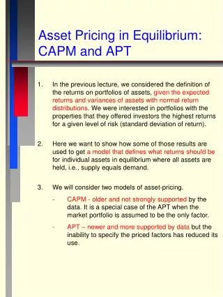
Asset Pricing in Equilibrium:CAPM and APT • In the previous lecture, we considered the definition of the returns on portfolios of assets, given the expected returns and variances of assets with normal return distributions. We were interested in portfolios with the properties that they offered investors the highest returns for a given level of risk (standard deviation of return). • Here we want to show how some of those results are used to get a model that defines what returns should be for individual assets in equilibrium where all assets are held, i.e., supply equals demand. • We will consider two models of asset-pricing. • CAPM - older and not strongly supported by the data. It is a special case of the APT when the market portfolio is assumed to be the only factor. • APT – newer and more supported by data but the inability to specify the priced factors has reduced its use.
Assumptions for CAPM • Investors are risk averse and maximize expected utility of end-of-period wealth. • Investors are price takers with homogeneous expectations about joint normal asset returns. • A risk-free asset exists with borrowing and lending. • Asset quantities are fixed, assets are marketable and divisible. • Asset markets are frictionless with information available costlessly to all instantaneously. • No taxes, regulations and short-selling restrictions.
3. These assumptions may seem reasonable because they are frequently used in many other economic models. In fact, I believe that the assumptions of costless information and homogeneous expectations are too strong. The purpose of a market is to provide a means for trade, however, if everyone sees assets the same way, there is little reason for individuals to trade assets except for liquidity reasons. 4. The reasoning underlying the CAPM is somewhat circular. Since we know everyone sees assets the same wayand each chooses an efficient portfolio, then since the market portfolio is just a combination of these efficient portfolios, the marketportfolio will also be efficient. The efficiency of the market portfolio is the primary testable implication of the CAPM but because the market portfolio includes all assets and data on all assets is unavailable, the CAPM is largely untestable.
Derivation of the CAPM Consider the market portfolio M consisting of all assets. The weighting of each asset i in the market portfolio is Wi = (market value of asset i)/(Market value of all assets) 1. Form a portfolio of a% of the risky asset i and (1-a)% of the market portfolio, its mean and standard deviation are E(Rp) = aE(Ri) + (1-a)E(Rm) (Rp) = [a2i2 + (1-a)2m2 + 2a(1-a)im].5 2. Now define the change in each of these with respect to a change in the weight a, E(Rp)/a = E(Ri) - E(Rm) (Rp)/a = .5[a2i2 + (1-a)2m2 + 2a(1-a)im]-.5 x [2ai2 - 2m2 + 2am2 + 2im – 4aim] 3. This is equivalent to saying, “consider the market portfolio and assume we increase the weight a of asset i in the market portfolio”. But if we add more asset i, by definition we are no longer in equilibrium since the market portfolio is an equilibrium portfolio. Thus, in equilibrium, a = 0.
Assuming a=0, then the previous derivatives are E(Rp)/a = E(Ri) - E(Rm) (Rp)/a = .5[m2]-.5[ - 2m2 + 2im ] = [im - m2 ]/ m 4. The risk-return tradeoff evaluated at point M is thus [E(Rp)/a]/[(Rp)/a] = [E(Ri) - E(Rm)]/{[im - m2 ]/ m} This defines the equilibrium risk-return trade-off. This is the marginal return (marginal benefit to investor) offered for marginal risk (marginal cost to investor) in equilibrium. 5. The slope of the investment opportunity set defined by asset i and the market portfolio must be equal to the slope of the capital market line (because the frontier defined by i and M is a parabola that includes M). Assuming efficiency, the portfolio tangent to the CML must be the market portfolio M. Capital Market Line Slope = [E(Rm) - Rf]/ m Therefore, [E(Ri) - E(Rm)]/{[im - m2 ]/ m} = [E(Rm) - Rf]/ m Solve for E(Ri) E(Ri) = Rf + [E(Rm) - Rf] im/m2
This defines the Security Market Line (CAPM) where the required return, E(Ri), of any security must fall on the line that begins at Rf, has a slope of [E(Rm) - Rf] and a domain over • i = im/m2 . • measures the units of risk for a particular asset. 6. Therefore, an asset’s return equals the risk-free return if = 0, i.e., its returns are uncorrelated with that of the market’s. E(Ri) = Rf if i = 0 E(Ri) = Rf + [E(Rm) - Rf]iif i 0 E(Ri) = risk-free return + (price of unit of risk)(units of risk) 7. The main implication of the CAPM is that all assets should plot along the Security market line in (E(R), ) space. Contrast this with what we had from the previous lecture that all assets plot somewhere within or on a parabola in (E(R), ) , with the edge of the parabola defined by the minimum variance for a given return.
8. What explains the difference between results for (E(R), ) space and (E(R), ) space ? Consider what we call the Market Model. Ri = ai + biRm + ei It relates the return on the asset to the market return in a regression where e is assumed to be an independent error term. (versions of this are often used in empirical studies). Assuming normal distributions, we can define the return variance as i2 = bi2m2 + e2 Here, the first term on the RHS is the market-related variance, called nondiversifiable risk and the second term in asset-specific variance or diversifiable risk. One can show that bi = i so that beta defines an asset’s nondiversifiable portion of return variance, however, the diversifiable portion differs for different assets, therefore, even though all assets plot on a line in (E(R), ) space, they are more spread out in (E(R), ) space. Because no one will pay higher returns to those bearing more diversifiable variance, assets that have the same betas will have the same expected return even though some have larger variances than others. 9. To get the risk of a portfolio of assets, one can simply take the weighted average of the betas, where the weights are the proportions of the total portfolio placed in each asset .
Applications and Extensions • Conditional CAPM - The derivation of the CAPM above is in a one-period context. In an intertemporal (multiperiod) context, things can change. In particular, unless we assume that a company’s risk does not change over time, then Beta will change and this adds additional uncertainty to the model. • The CAPM Model can be restated in intertemporal form • Et-1 Rit = Rft + Bit-1 Et-1 [Rmt -Rft ] • Where Bit-1 = Covt-1(Rit , Rmt )/Var(Rmt) • To get unconditional expectations we us the Law of Iterated Expectations to get • Et-1 E(Rit) = Rft + E(Bit-1 Et-1 [Rmt -Rft ]) • Which equals • E(Rit) = Rft + E(Bit-1 Et-1 [Rmt -Rft ]) • From the definition of covariance we can substitute for the expectation of a product of random variables to get • E(Rit) = Rft + E(Bit-1)Et-1 [Rmt -Rft ] + Cov(Bit-1, Et-1 [Rmt -Rft ]) • Now, this ICAPM looks similar to the CAPM except for an additional term that measures the degree to which a company’s beta moves with the market risk premium.
The extra term can be explained as follows. Consider two assets with the same unconditional betas (E(Bit-1)), that is, the same average beta over the full range of the economic cycle. Asset 1, whose beta tends to be larger than average in good times (when Et-1[Rmt - Rft ] is large) but smaller in bad times should have a larger expected return. Note that Et-1[Rmt - Rft ]is always positive so the asset will earn less in the bad times because its beta is smaller than average in bad times. This asset is riskier than asset 2 whose beta stays fixed at the average over time. That asset earns more in the bad times than the asset 1. • The CAPM is often used to estimate a company’s cost of equity. • a. First, estimate a company’s beta with the market model and 3-5 years of return data on the stock and the market portfolio (usually the S&P 500). • b. Next, assume that the risk-free rate is the long-term U.S. Treasury bond rate, now at about 6%. • c. Also assume that the expected market return is, say 12%, which is the average return on the S&P 500 over the last 70 years. • d. Plug these numbers into the CAPM, e.g. • ki = .06 + 1.2[.12 - .06] = .132 for i = 1.2
2. There are many extensions of the CAPM. Most are associated with relaxing one of the assumptions. For example, human capital is not tradable (no slavery) so the model has been derived under the conditions of untradable assets. The most important extension involves the case where no riskless asset exists. When no riskless asset exists, we can still find a minimum variance portfolio for which = 0, and the return on this portfolio Rz can be substituted for the riskless rate in the CAPM. All of the properties of the CAPM, like linearity and beta as the risk measure, still hold. This form of the of the CAPM is called the two-factor model. Recall from the previous lecture that any portfolio on the efficient frontier could be seen as a combination of the minimum variance portfolio and another portfolio on the frontier. Here, the other portfolio is the market portfolio. 3.Other types of extensions of the CAPM are typically solved by adding another portfolio to the model in addition to the market portfolio. Then we will get, say, three fund separation. The extra fund is part of the CAPM in order to allow for a new risk to be hedged. For example, a portfolio that captures the covariance between the market portfolio and untraded human capital allows individuals to either reduce their human capital risk (short the portfolio) or increase it (purchase the portfolio). Something like APT with a human capital factor.
4.The most damaging assumption is the assumption that investors have homogeneous expectations. When this assumption does not hold, the market portfolio will be inefficient and thus the CAPM is not testable. • 5.Early tests of the CAPM supported the model but most recent tests have rejected it. One study showed that earlier studies largely relied on a unique sample period where the model fit well – in other samples it performs poorly. • 6.Roll’s critique of the CAPM suggests that • To test the CAPM we need data on all assets in the market portfolio and one must show that the market portfolio is efficient. This is nearly impossible to do. • If we use an ex post efficient portfolio to measure investment performance, then efficient set mathematics implies that no security will have abnormal performance – all will lie on the SML. • If we use an ex post inefficient set to measure performance, any result is possible so no inference concerning performance should be made. This means that if we find that all assets (don’t) lie on the SML, the CAPM is supported (rejected) assuming we measured the market portfolio correctly, or we could have gotten lucky (unlucky) with an incorrect market portfolio.
7. What underlies Roll’s critique is found in the previous class on selection of the investment opportunity set. NOTE: The definitions of the scalars have been changed to Ingersol’s (1987, p. 84) definitions. 7a. When there are many assets instead of just two we get, p2 = [A2 – 2B + C]/D Where A = 1’-11 > 0, B = 1’-1E, C = E’ -1E > 0, D=AC – B2 > 0 and -1 is the inverse of the variance-covariance matrix of returns and E is the vector of expected returns. This is also a parabola. 7b. The portfolio weights (wi) which are very complex can be represented more easily for the general case of many assets in matrix form as follows. W = -11/A + -1E/B where = A[C – B]/D and = B[A – B]/D. One can show that + = 1. Also note that this shows that the weights are functions of the minimum variance portfolio [1/A] and the portfolio represented by [E/B]. This will be called “two fund separation”. 7c. Roll’s point: portfolio [E/B] can be any efficient portfolio and [1/A] is its associated minimum variance portfolio
8.Why is the only test of the model a test of the efficiency of the market portfolio? Because the model is an “equilibrium” model it requires that supply equals demand for all assets. This implies that the weight of each asset in the market portfolio is its value as a percent of total market value. With homogeneous expectation assumed, then we know all investors view asset distributions the same and will hold assets in a way to minimize the variance of their returns. This requires everyone to have the same portfolio weights for the risky assets they hold. Summed across individuals, this happens only when the asset weights equal their percent of total market asset value. Equilibrium and homogeneous expectations severely limit the number of observable implications of the model.Thus, the only testable proposition is to see whether the market portfolio is efficient, i.e., ex ante, could investors do better if they held their risky assets in some other portfolio.
Hansen-Jagannathan (1991 JPE) lower bound condition on asset pricing kernel (SDF) and relation to risk-free and risk premium puzzles. The price of a simple security at time t (Pt) that pays an uncertain cash flow at time t+1 (Xt+1) is: Pt = Et[dt+1Xt+1] where dt+1 is the stochastic discount factor.(SDF) Note that dt+1 is random because it depends upon the random amount of consumption in t+1. If consumption is high in t+1, then dt+1 will be small because the marginal utility of consumption in t+1 will be small. This makes the asset price small because consumers value the cash flow Xt+1 less. Any asset is priced according to the cash flow it provides multiplied by the same dt+1, hence, the SDF is called a pricing kernel. Note that the expectation of dt+1 equals the risk free discount rate (1/(1 + Rf)) because across all states, the average return equals the risk free rate. That is, form a portfolio by purchasing one state security for each possible state. The return for that portfolio equals the risk free rate.
Hansen-Jagannathan (1991 JPE) lower bound condition on asset pricing kernel (SDF) and relation to risk-free and risk premium puzzles. If we divide through by current time t price to get return 1 = Et[dt+1Rt+1] This holds for all states of nature so it holds unconditionally and for any two assets such as the market portfolio (m) and risk free asset (f), or the difference between them is: E[d(Rm – Rf)] = 0 or E(d)E(Rm-Rf) + cov(d, Rm-Rf) = 0 And after substitutions for cov and rearranging E(Rm-Rf)/m-f = -ρd,mf[d/E(d)] Because correlation cannot exceed |1| then, d/E(d) = d(1 + Rf) > | E(Rm-Rf)/m-f | For the CCAPM the SDF is the MRS of current for future consumption and its expectation equals 1/(1+Rf) which equals say, 0.96 (Rf=0.04). The average risk premium equals 0.062 and has a standard deviation of 0.167. This implies that d > 0.96(0.062/0.167) = 0.355 But measured standard deviation of d is much lower at 0.002. The stand. dev. Is small because consumption is smooth. This might hold if Rf was much larger or Rm-Rf was much smaller. These are called the risk free rate and risk premium puzzles.
APT – Arbitrage Pricing • 1.Assumptions • Perfect competition and frictionless markets. • The number of assets n must be much larger than the number of factors that generate returns. • The unsystematic risk component of asset i is ei. It must be independent of all factors and all other assets’ ej. • d. Investors have homogeneous beliefs that asset returns are governed by a linear k-factor model such as • Ri = E(Ri) + i = E(Ri) + bi1F1 + bi2F2 + …. + bikFk + ei • where Ri = asset i’s random return. • E(Ri) = asset i’s expected return. • bik = the sensitivity of asset i’s return to the kth factor. • Fk = the mean zero kth common factor (non-zero factors can be restated as deviations from their mean) • i, ei = the mean zero error terms for asset i. • 2. The APT relies on the simple concept of arbitrage. The no-arbitrage condition states that in equilibrium, portfolios of assets with • No net investment – i.e., some assets purchased and some assets sold short. • No net risk – i.e. no probability of loss should earn no return. Otherwise, infinite riskless returns are available.
Interpreting the APT Return-Generating Model The linear k-factor model is: Ri = E(Ri) + i = E(Ri) + bi1F1 + bi2F2 + …. + bikFk + ei It generates the actual return for a particular period, e.g. day. It says that stock i’s return today will be its expected return as long as the realized values of all the factors equals their expected values of zero, and the firm-specific return e is zero. Of course, the F and e are random, so the actual return for a particular day will depend on their realized values as well as a firm’s factor betas b. This holds also for the CAPM model with the market return Rm as: Ri = E(Ri) + B[Rm – E(Rm)] + ei Here the market return is demeaned to give a zero mean factor. The APT is a model of expected returns, not actual returns. Below we will derive a two factor APT from the return generating model above to get. E(Ri) = Rf + [E(RM) - Rf ]biM + [E(RO) - Rf ]biO The factor risk premiums are in square brackets and a particular firm’s factor loadings (betas) are applied to the premiums to obtain its expected return. Note that the Fama-French factor data are zero investment portfolio returns but they are not mean zero returns. For the size factor, you go long small and short large to get: {.5[E(Rs) – Rf] - .5[E(RL) – Rf]} = .5[E(Rs) – E(RL)].
Derivation of APT • Create an arbitrage portfolio. Let wi be the change in the dollar amount invested in asset i as a percentage of an individual’s wealth. Then the summation over longs and shorts balance so • iwi = 0. • 2. The returns on this portfolio are then • Portfolio Return = Rp = iwiRi • = iwiE(Ri) + iwibi1F1 + iwibi2F2 + …. + iwibikFk + iwiei • 3. Select the the weights wi so as to eliminate both systematic and unsystematic risk. This can be done by selecting • wi = 1/n with n large • and iwibik = 0 for each factor k. • This means wi is tiny, and that the arbitrage portfolio “betas” for each factor are zero, so that all risk is eliminated and • Portfolio Return = Rp = iwiRi = iwiE(Ri) • 4. If markets are in equilibrium then Rp = iwiRi = iwiE(Ri) =0. This riskless portfolio, requiring no net investment, must earn zero return because, otherwise, everyone would want to own the portfolio and prices would change – contradicting the assumption of equilibrium.
5. Restated using vectors we have: w’1 = 0, w’bk = 0 for each factor k, implies w’E = 0 where E is the vector of expected returns. A theorem in linear algebra states that if the fact that a vector (here, w) is orthogonal to k+1 vectors (here, 1 and each of k vectors bk ) implies it is orthogonal to another vector (here, E) then this other vector can be expressed as a linear combination of the first k+1 vectors. This implies that E(Ri) = 01 + 1bi1 + 2bi2 + …. + kbik Here, the i represent the price of risk specific to each factor k. 6. An intuitive restatement: When we selected a portfolio with w’1 = 0 and w’bk = 0 for each factor k, we know that we have spanned the expected return space because w’E = 0. w’E = 0 means that there are no net returns to this portfolio, i.e., there is nothing left in the vector of expected returns to be explained. Therefore, it must be that E is simply a linear combination of the vector 1 and the k vectors bk. Of course, this is not so surprising. We started by assuming that all investors believed that asset returns are governed by a linear model with k factors. This just proves that greedy, risk averse investors will, in fact, price assets to reflect these factor risks. If they don’t, then arbitrage is possible.
7. A riskless asset has bik = 0 for all k so that Rf = 0 And therefore E(Ri) = Rf + 1bi1 + 2bi2 + …. + kbik 8. Suppose we assume that the only risk factor is the general market risk represented by the market portfolio M and returns are joint normal, then E(Ri) = Rf + MbiM This is just the CAPM where the units of risk are biM = i and the price per unit of risk is M = [E(RM) - Rf ]. To see how this comes about, note that this must hold for the market portfolio itself, which has a biM = i =1. Therefore, E(RM) = Rf + M(1) Or M = [E(RM) - Rf ]. Now we are back to the CAPM where for any asset i, E(Ri) = Rf + [E(RM) - Rf ]biM
9. Now suppose there are 2 factors, the market portfolio and oil prices. The APT requires that expected returns follow E(Ri) = Rf + MbiM + ObiO We can select a portfolio such that it has biO =1 but biM = 0. This portfolio must also follow the relationship so that E(RO) = Rf + M(0) + O(1) Or O = [E(RO) - Rf ] The two factor APT for the expected return of any asset i is E(Ri) = Rf + [E(RM) - Rf ]biM + [E(RO) - Rf ]biO 10. More generally for factors numbered 1 to k, select k portfolios such that each loads only on one factor, that is, each portfolio’s return can represent the return on a factor. E(Ri) = Rf + [E(R1) - Rf ]bi1 + [E(R2) - Rf ]bi2 + … + [E(Rk) - Rf ]bik The notation often used is to have k = E(Rk) which gives E(Ri) = Rf + [1 - Rf ]bi1 + [2 - Rf ]bi2 + … + [k - Rf ]bik Like the CAPM beta, each bik = ik/ k2
In a one factor APT depicted above, the expected return (i) - risk (bi) combinations for all of the assets must lie on a line that passes through rf. Thus all assets must fall on this Security Market Line or else arbitrage exists. In the case above, we would sell short a portfolio of assets 1 and 3 which has a risk level of b2. Then take the short sale proceeds and purchase asset 2. This portfolio is riskless but should produce a positive return. If APT is correct, this should not be possible.
Advantages of the APT Over the CAPM • No assumptions about return distributions. • No assumptions on utility except greed and risk aversion. • APT applies to any subset of assets – don’t need to know the return distribution of all assets. • No special role for the market portfolio – easier testing. • Easy to extend to multi-period framework. • Most important: Many factors can impact returns – if the risk-return world is multi-faceted, using only the market return will give poorer return predictions – like being in a plane trying to land and offered only the fact that you are 200 miles from the destination (no latitude, longitude or altitude). • For example, some Wall Street investment banks used CAPM type models to determine that some Japanese stock warrants were under-priced. They bought the warrants and hedged using Japanese futures. Unfortunately, more than just a market factor was important so their hedges worked poorly and they lost.
Problems and Applications • Major empirical problem: the factors are not specified, making testing more difficult. Some factors people have used are • Industrial production • Changes in default risk premiums (AAA – Baa) • Yield curve (Long – short treasury yields) • Unanticipated inflation • 2. Like the CAPM, the APT can be used to estimate the cost of equity for a firm given its betas on the factors. • 3. The factor betas for a portfolio are just a linear combination of the individual asset betas with their value weights.