Chapter 7 Sorting: Outline
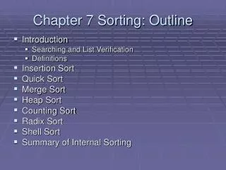
Chapter 7 Sorting: Outline. Introduction Searching and List Verification Definitions Insertion Sort Quick Sort Merge Sort Heap Sort Counting Sort Radix Sort Shell Sort Summary of Internal Sorting. Introduction (1/9). Why efficient sorting methods are so important ?

Chapter 7 Sorting: Outline
E N D
Presentation Transcript
Chapter 7 Sorting: Outline • Introduction • Searching and List Verification • Definitions • Insertion Sort • Quick Sort • Merge Sort • Heap Sort • Counting Sort • Radix Sort • Shell Sort • Summary of Internal Sorting
Introduction (1/9) • Why efficient sorting methods are so important ? • The efficiency of a searching strategy depends on the assumptions we make about the arrangement of records in the list • No single sorting technique is the “best” for all initial orderings and sizes of the list being sorted. • We examine several techniques, indicating when one is superior to the others.
Introduction (2/9) • Sequential search • We search the list by examining the key values list[0].key, … , list[n-1].key. • Example: List has n records.4, 15, 17, 26, 30, 46, 48, 56, 58, 82, 90, 95 • In that order, until the correct record is located, or we have examined all the records in the list • Unsuccessful search: n+1 O(n) • Average successful search
[6] [5] [1] [3] [8] [0] [2] 15 4 46 48 17 58 26 [10] 90 [4] [7] [9] [11] 30 56 82 95 Introduction (3/9) • Binary search • Binary search assumes that the list is ordered on the key field such that list[0].key list[1]. key … list[n-1]. key. • This search begins by comparing searchnum (search key) and list[middle].key where middle=(n-1)/2 4, 15, 17, 26, 30, 46, 48, 56, 58, 82, 90, 95 Figure 7.1:Decision tree for binary search (p.323)
Introduction (4/9) • Binary search (cont’d) • Analysis of binsearch: makes no more than O(log n) comparisons
Introduction (5/9) • List Verification • Compare lists to verify that they are identical or identify the discrepancies. • Example • International Revenue Service (IRS) (e.g., employee vs. employer) • Reports three types of errors: • all records found in list1 but not in list2 • all records found in list2 but not in list1 • all records that are in list1 and list2 with the same key but have different values for different fields
Introduction (6/9) • Verifying using a sequential search Check whether the elements in list1 are also in list2 And the elements in list2 but not in list1 would be show up
Introduction (7/9) • Fast verification of two lists The element of list1 is not in list2 The element of two lists are matched The element of list2 is not in list1 The remainder elements of a list is not a member of another list
Introduction (8/9) • Complexities • Assume the two lists are randomly arranged • Verify1: O(mn) • Verify2: sorts them before verificationO(tsort(n) + tsort(m) + m + n) O(max[nlogn, mlogm]) • tsort(n): the time needed to sort the n records in list1 • tsort(m): the time needed to sort the m records in list2 • we will show it is possible to sort n records in O(nlogn) time • Definition • Given (R0, R1, …, Rn-1), each Ri has a key value Kifind a permutation , such that K(i-1) K(i), 0<i n-1 • denotes an unique permutation • Sorted: K(i-1) K(i), 0<i<n-1 • Stable: if i < j and Ki = Kj then Ri precedes Rj in the sorted list
Introduction (9/9) • Two important applications of sorting: • An aid to search • Matching entries in lists • Internal sort • The list is small enough to sort entirely in main memory • External sort • There is too much information to fit into main memory
Insertion Sort (1/3) • Concept: • The basic step in this method is to insert a record R into a sequence of ordered records, R1, R2, …, Ri (K1 K2 , …, Ki) in such a way that the resulting sequence of size i is also ordered • Variation • Binary insertion sort • reduce search time • List insertion sort • reduce insert time
Insertion Sort (2/3) list [0] [1] [2] [3] [4] • Insertion sort program 1 2 5 3 2 2 5 3 5 3 5 1 4 4 5 i = 4 3 1 2 next = 3 1 4 2
Insertion Sort (3/3) • Analysis of InsertionSort: • If k is the number of records LOO, then the computing time is O((k+1)n) • The worst-case time is O(n2). • The average time is O(n2). • The best time is O(n). left out of order (LOO) O(n)
Quick Sort (1/6) • The quick sort scheme developed by C. A. R. Hoare has the best average behavior among all the sorting methods we shall be studying • Given (R0, R1, …, Rn-1) and Kidenote a pivot key • If Ki is placed in position s(i),then Kj Ks(i)for j < s(i), Kj Ks(i)for j > s(i). • After a positioning has been made, the original file is partitioned into two subfiles, {R0, …, Rs(i)-1}, Rs(i), {Rs(i)+1, …, Rs(n-1)}, and they will be sorted independently
Quick Sort (2/6) • Quick Sort Concept • select a pivot key • interchange the elements to their correct positions according to the pivot • the original file is partitioned into two subfiles and they will be sorted independently R0 R1 R2 R3 R4 R5 R6 R7 R8 R9 26 5 37 1 61 11 59 15 48 19 11 5 19 1 15 26 59 61 48 37 1 5 11 19 15 26 59 61 48 37 1 5 11 19 15 26 59 61 48 37 1 5 11 15 19 26 59 61 48 37 1 5 11 15 19 26 48 37 59 61 1 5 11 15 19 26 37 48 59 61 1 5 11 15 19 26 37 48 59 61
a 6 6 2 8 8 5 11 10 4 1 9 7 3 3 a 6 6 2 3 5 11 11 10 4 1 1 9 7 8 a 6 6 2 3 5 1 10 10 4 4 11 9 7 8 a 6 6 2 3 5 1 4 4 10 10 11 9 7 8 a 4 2 3 5 1 4 6 6 10 11 9 7 8 In-Place Partitioning Example bigElement is not to left of smallElement, terminate process. Swap pivot and smallElement.
Quick Sort (4/6) • Analysis for Quick Sort • Assume that each time a record is positioned, the list is divided into the rough same size of two parts. • Position a list with n element needs O(n) • T(n) is the time taken to sort n elements • T(n)<=cn+2T(n/2) for some c <=cn+2(cn/2+2T(n/4)) ... <=cnlog2n+nT(1)=O(nlogn) • Time complexity • Average case and best case: O(nlogn) • Worst case: O(n2) • Best internal sorting method considering the average case • Unstable
Quick Sort (5/6) • Lemma 7.1: • Let Tavg(n) be the expected time for quicksort to sort a file with n records. Then there exists a constant k such that Tavg(n) knlogen for n 2 • Space for Quick Sort • If the smaller of the two subarrays is always sorted first, the maximum stack space is O(logn) • Stack space complexity: • Average case and best case: O(logn) • Worst case: O(n)
Quick Sort (6/6) • Quick Sort Variations • Quick sort using a median of three: Pick the median of the first, middle, and last keys in the current sublist as the pivot. Thus, pivot = median{Kl, K(l+r)/2, Kr}.
a a 6 3 2 2 3 8 6 3 10 10 3 10 6 10 3 8 5 5 11 11 10 10 4 4 1 1 9 9 7 7 3 6 a a 3 3 2 2 8 1 5 5 4 11 6 6 11 4 8 1 9 9 7 7 10 10 6 a 3 3 2 5 11 7 4 6 10 10 6 8 1 9 a 3 3 2 1 5 7 8 9 6 10 10 6 11 4 a 3 3 2 1 5 11 8 9 6 10 10 6 4 7 6 Median of Three Partitioning Example
Merge Sort (1/7) • Before looking at the merge sort algorithm to sort n records, let us see how one may merge two sorted lists to get a single sorted list. • Merging • Uses O(n) additional space. • It merges the sorted lists (list[i], … , list[m]) and (list[m+1], …, list[n]), into a single sorted list, (sorted[i], … , sorted[n]). • Copy sorted[1..n] to list[1..n]
Merge Sort (3/7) • Recursive merge sort concept
Merge Sort (4/7) • Recursive merge sort concept
Merge Sort (5/7) • Recursive merge sort concept
Merge Sort (6/7) • Recursive merge sort concept
Merge Sort (7/7) • Recursive merge sort concept
Heap Sort (1/3) • The challenges of merge sort • The merge sort requires additional storage proportional to the number of records in the file being sorted. • Heap sort • Require only a fixed amount of additional storage • Slightly slower than merge sort using O(n) additional space • The worst case and average computing time is O(n log n), same as merge sort • Unstable
root = 1 n = 10 • adjust • adjust the binary tree to establish the heap rootkey = 26 child = 6 7 3 2 14 /* compare root and max. root */ [1] 77 26 /* move to parent */ 5 59 77 [2] [3] 1 61 11 26 59 [4] [5] [6] [7] 15 48 19 [8] [9] [10]
Heap Sort (3/3) • heapsort n = 10 i = 8 9 1 5 4 3 2 1 7 6 5 4 3 2 bottom-up ascending order(max heap) [1] 26 19 48 61 11 15 26 77 59 1 1 5 1 5 5 1 5 1 1 top-down 5 77 [2] 15 61 5 1 5 [3] 11 59 26 11 1 19 48 1 61 11 59 15 48 15 1 [4] [5] 19 19 5 26 1 [6] [7] 26 48 1 15 48 19 [8] 59 5 [9] 1 61 5 77 [10]
Counting Sort • For key values within small range • 1. scan list[1..n] to count the frequency of every value • 2. sum to find proper index to put value x • 3. scan list[1..n] and put to sorted[] • 4. copy sorted to list • O(n) for time and space
Radix Sort (1/5) • We considers the problem of sorting records that have several keys • These keys are labeled K0 (most significant key), K1, … , Kr-1 (least significant key). • Let Ki j denote key Kj of record Ri. • A list of records R0, … , Rn-1, is lexically sorted with respect to the keys K0, K1, … , Kr-1iff(Ki0, Ki1, …, Kir-1) (K0i+1, K1i+1, …, Kr-1i+1), 0 i < n-1
Radix Sort (2/5) • Example • sorting a deck of cards on two keys, suit and face value, in which the keys have the ordering relation:K0 [Suit]: < < < K1 [Face value]: 2 < 3 < 4 < … < 10 < J < Q < K < A • Thus, a sorted deck of cards has the ordering:2, …, A, … , 2, … , A • Two approaches to sort: • MSD (Most Significant Digit) first:sort on K0, then K1, ... • LSD (Least Significant Digit) first:sort on Kr-1, then Kr-2, ...
Radix Sort (3/5) • MSD first • MSD sort first, e.g., bin sort, four bins • LSD sort second • Result: 2, …, A, … , 2, … , A
Radix Sort (4/5) • LSD first • LSD sort first, e.g., face sort, 13 bins 2, 3, 4, …, 10, J, Q, K, A • MSD sort second (may not needed, we can just classify these 13 piles into 4 separated piles by considering them from face 2 to face A) • Simpler than the MSD one because we do not have to sort the subpiles independently Result: 2, …, A, … , 2, …, A
Radix Sort (5/5) • We also can use an LSD or MSD sort when we have only one logical key, if we interpret this key as a composite of several keys. • Example: • integer: the digit in the far right position is the least significant and the most significant for the far left position • range: 0 K 999 • using LSD or MSD sort for three keys (K0, K1, K2) • since an LSD sort does not require the maintainence of independent subpiles, it is easier to implement MSD LSD 0-9 0-9 0-9
Shell Sort • For (h = magic1; h > 0; h /= magic2) Insertion sort elements with distance h • Idea: let data has chance to “long jump” • Insertion sort is very fast for partially sorted array • The problem is how to find good magic? • Several sets have been discussed • Remember 3n+1
Summary of Internal Sorting (1/2) • Insertion Sort • Works well when the list is already partially ordered • The best sorting method for small n • Merge Sort • The best/worst case (O(nlogn)) • Require more storage than a heap sort • Slightly more overhead than quick sort • Quick Sort • The best average behavior • The worst complexity in worst case (O(n2)) • Radix Sort • Depend on the size of the keys and the choice of the radix
Summary of Internal Sorting (2/2) • Analysis of the average running times