Data Mining
Data Mining. What Is Data Mining?. Data Mining is the discovery of hidden knowledge, unexpected patterns and new rules in large databases Automating the process of searching patterns in the data. Objective of Data Mining. Any of four types of relationships are sought:

Data Mining
E N D
Presentation Transcript
Data Mining Flisha Fernandez
What Is Data Mining? • Data Mining is the discovery of hidden knowledge, unexpected patterns and new rules in large databases • Automating the process of searching patterns in the data Emily Thomas, State University of New York
Objective of Data Mining • Any of four types of relationships are sought: • Classes – stored data is used to locate data in predetermined groups • Clusters – data items grouped according to logical relationships or consumer preferences • Associations – Walmart example (beer and diapers) • Sequential Patterns – data mined to anticipate behavior patterns and trends anderson.ucla.edu
Data Mining Techniques • Rule Induction – extraction of if-then rules • Nearest Neighbors • Artificial Neural Networks – models that learn • Clustering • Genetic Algorithms – concept of natural evolution • Factor Analysis • Exploratory • Stepwise Regression • Data Visualization – usage of graphic tools • Decision Trees Emily Thomas, State University of New York
Classification • A major data mining operation • Given one attribute (e.g. Wealth), try to to predict the value of new people’s wealths by means of some of the other available attributes • Applies to categorical outputs • Categorical attribute: an attribute which takes on two or more discrete values, also knows as a symbolic attribute • Real attribute: a column of real numbers, also known as a continuous attribute Flisha Fernandez
Dataset real symbol classification Kohavi 1995
Decision Trees Flisha Fernandez
Decision Trees • Also called classification trees or regression trees • Based on recursive partitioning of the sample space • Tree-shaped structures that represent sets of decisions/data which generate rules for the classification of a (new, unclassified) dataset • The resulting classification tree becomes an input for decision making anderson.ucla.edu / Wikipedia
Decision Trees • A Decision Tree is where: • The nonleaf nodes are labeled with attributes • The arcs out of a node labeled with attribute Aare labeled with each of the possible values of the attribute A • The leaves of the tree are labeled with classifications Learning Decision Trees
Advantages • Simple to understand and interpret • Requires little data preparation (other techniques need data normalization, dummy variables, etc.) • Can support both numerical and categorical data • Uses white box model (explained by boolean logic) • Reliable – possible to validate model using statistical tests • Robust – large amounts of data can be analyzed in a short amount of time Wikipedia
Decision Tree Example Flisha Fernandez
David’s Debacle • Status Quo: Sometimes people play golf, sometimes they do not • Objective: Come up with optimized staff schedule • Means: Predict when people will play golf, when they will not From Wikipedia
David’s Dataset Quinlan 1989
David’s Diagram outlook? From Wikipedia humid? windy?
David’s Decision Tree Root Node Non-leaf Nodes Labeled with Attributes Arcs Labeled with Possible Values Sunny Rain Overcast Flisha Fernandez Normal High False True Leaves Labeled with Classifications
David’s Decision • Dismiss staff when it is • Sunny AND Hot • Rainy AND Windy • Hire extra staff when it is • Cloudy • Sunny AND Not So Hot • Rainy AND Not Windy From Wikipedia
Decision Tree Induction Flisha Fernandez
Decision Tree Induction Algorithm • Basic Algorithm (Greedy Algorithm) • Tree is constructed in a top-down recursive divide-and-conquer manner • At start, all the training examples are at the root • Attributes are categorical (if continuous-valued, they are discretized in advance) • Examples are partitioned recursively based on selected attributes • Test attributes are selected on the basis of a certain measure (e.g., information gain) Simon Fraser University, Canada
Issues • How should the attributes be split? • What is the appropriate root? • What is the best split? • When should we stop splitting? • Should we prune? Decision Tree Learning
Two Phases • Tree Growing (Splitting) • Splitting data into progressively smaller subsets • Analyzing the data to find the independent variable (such as outlook, humidity, windy) that when used as a splitting rule will result in nodes that are most different from each other with respect to the dependent variable (play) • Tree Pruning DBMS Data Mining Solutions Supplement
Splitting Flisha Fernandez
Splitting Algorithms • Random • Information Gain • Information Gain Ratio • GINI Index DBMS Data Mining Solutions Supplement
Dataset AIXploratorium
Random Splitting AIXploratorium
Random Splitting • Disadvantages • Trees can grow huge • Hard to understand • Less accurate than smaller trees AIXploratorium
Splitting Algorithms • Random • Information Gain • Information Gain Ratio • GINI Index DBMS Data Mining Solutions Supplement
Information Entropy • A measure of the uncertainty associated with a random variable • A measure of the average information content the recipient is missing when they do not know the value of the random variable • A long string of repeating characters has an entropy of 0, since every character is predictable • Example: Coin Toss • Independent fair coin flips have an entropy of 1 bit per flip • A double-headed coin has an entropy of 0 – each toss of the coin delivers no information Wikipedia
Information Gain • A good measure for deciding the relevance of an attribute • The value of Information Gain is the reduction in the entropy of X achieved by learning the state of the random variable A • Can be used to define a preferred sequence (decision tree) of attributes to investigate to most rapidly narrow down the state of X • Used by ID3 and C4.5 Wikipedia
Calculating Information Gain • First compute information content • Ex. Attribute Thread = New, Skips = 3, Reads = 7 • -0.3 * log 0.3 - 0.7 * log 0.7 • = 0.881 (using log base 2) • Ex. Attribute Thread = Old, Skips = 6, Reads = 2 • -0.6 * log 0.6 - 0.2 * log 0.2 • = 0.811 (using log base 2) • Information Gain is... • Of 18, 10 threads are new and 8 threads are old • 1.0 - (10/18)*0.881 + (8/18)*0.811 • 0.150 Flisha Fernandez
Information Gain AIXploratorium
Test Data AIXploratorium
Drawbacks of Information Gain • Prefers attributes with many values (real attributes) • Prefers AudienceSize {1,2,3,..., 150, 151, ..., 1023, 1024, ... } • But larger attributes are not necessarily better • Example: credit card number • Has a high information gain because it uniquely identifies each customer • But deciding how to treat a customer based on their credit card number is unlikely to generalize customers we haven't seen before Wikipedia / AIXploratorium
Splitting Algorithms • Random • Information • Information Gain Ratio • GINI Index DBMS Data Mining Solutions Supplement
Information Gain Ratio • Works by penalizing multiple-valued attributes • Gain ratio should be • Large when data is evenly spread • Small when all data belong to one branch • Gain ratio takes number and size of branches into account when choosing an attribute • It corrects the information gain by taking the intrinsic information of a split into account (i.e. how much info do we need to tell which branch an instance belongs to) http://www.it.iitb.ac.in/~sunita
Dataset http://www.it.iitb.ac.in/~sunita
Calculating Gain Ratio • Intrinsic information: entropy of distribution of instances into branches • Gain ratio (Quinlan’86) normalizes info gain by http://www.it.iitb.ac.in/~sunita
Computing Gain Ratio • Example: intrinsic information for ID code • Importance of attribute decreases as intrinsic information gets larger • Example of gain ratio: http://www.it.iitb.ac.in/~sunita
Dataset http://www.it.iitb.ac.in/~sunita
Information Gain Ratios http://www.it.iitb.ac.in/~sunita
More on Gain Ratio • “Outlook” still comes out top • However, “ID code” has greater gain ratio • Standard fix: ad hoc test to prevent splitting on that type of attribute • Problem with gain ratio: it may overcompensate • May choose an attribute just because its intrinsic information is very low • Standard fix: • First, only consider attributes with greater than average information gain • Then, compare them on gain ratio http://www.it.iitb.ac.in/~sunita
Information Gain Ratio • Below is the decision tree AIXploratorium
Test Data AIXploratorium
Splitting Algorithms • Random • Information • Information Gain Ratio • GINI Index DBMS Data Mining Solutions Supplement
GINI Index • All attributes are assumed continuous-valued • Assumes there exist several possible split values for each attribute • May need other tools, such as clustering, to get the possible split values • Can be modified for categorical attributes • Used in CART, SLIQ, SPRINT Flisha Fernandez
GINI Index • If a data set T contains examples from n classes, gini index, gini(T) is defined aswhere pj is the relative frequency of class j in node T • If a data set T is split into two subsets T1 and T2 with sizes N1 and N2 respectively, the gini index of the split data contains examples from n classes, the gini index gini(T) is defined as • The attribute that provides the smallest ginisplit(T) is chosen to split the node khcho@dblab.cbu.ac.kr
GINI Index • Maximum (1 - 1/nc) when records are equally distributed among all classes, implying least interesting information • Minimum (0.0) when all records belong to one class, implying most interesting information khcho@dblab.cbu.ac.kr
Examples for Computing Gini P(C1) = 0/6 = 0 P(C2) = 6/6 = 1 Gini = 1 – P(C1)2 – P(C2)2 = 1 – 0 – 1 = 0 khcho@dblab.cbu.ac.kr P(C1) = 1/6 P(C2) = 5/6 Gini = 1 – (1/6)2 – (5/6)2 = 0.278 P(C1) = 2/6 P(C2) = 4/6 Gini = 1 – (2/6)2 – (4/6)2 = 0.444
Stopping Rules • Pure nodes • Maximum tree depth, or maximum number of nodes in a tree • Because of overfitting problems • Minimum number of elements in a node considered for splitting, or its near equivalent • Minimum number of elements that must be in a new node • A threshold for the purity measure can be imposed such that if a node has a purity value higher than the threshold, no partitioning will be attempted regardless of the number of observations DBMS Data Mining Solutions Supplement / AI Depot
Overfitting • The generated tree may overfit the training data • Too many branches, some may reflect anomalies due to noise or outliers • Result is in poor accuracy for unseen samples • Two approaches to avoid overfitting • Prepruning: Halt tree construction early—do not split a node if this would result in the goodness measure falling below a threshold • Difficult to choose an appropriate threshold • Postpruning: Remove branches from a “fully grown” tree—get a sequence of progressively pruned trees • Use a set of data different from the training data to decide which is the “best pruned tree” Flisha Fernandez
Pruning • Used to make a tree more general, more accurate • Removes branches that reflect noise DBMS Data Mining Solutions Supplement

