Download
1 / 13
150 likes | 234 Vues
Learn how to determine volume fraction transformed and manage overlap in isothermal processes using Avrami equation and TTT diagrams. Explore cases, mathematical devices, and practical applications.

E N D
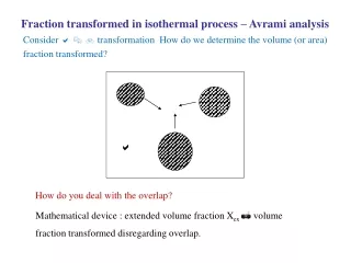
Fraction transformed in isothermal process – Avrami analysis Consider transformation How do we determine the volume (or area) fraction transformed? How do you deal with the overlap? Mathematical device : extended volume fraction Xex volume fraction transformed disregarding overlap.
Avrami equation The actual volume fraction grows in a relative amount to the unconsumed fraction, at the same rate the extended volume fraction does.: or Unconsumed fraction Integrate Expand : dilute overlap of two overlap of three
Case (1) constant number of heterogeneous nuclei present from the beginning. concentration: N growth rate of crystals : v x t Application to nucleation & growth : ( Johnson - Mehl) Plot of ln t vs ln[-ln(1-x)] should have slope of 3.
so Plot of ln t vs ln[-ln(1-x)] slope of 4 These plots are called Johnson- Mehl –Arami plots (JMA plots) Case (2) Assume a constant nucleation rate I, # of nuclei formed between t’ and t’ + dt’ ; concentration, N = I dt’ and at some later time ( t > t’ ) the “radius” of transformed phase is v (t – t’)
329K power DSC isothermals X 328K 328K 327K 325K 324K 326K 329K 1 327K 326K 325K 1/2 324K 20 40 60 80 100 0 Time (min) Time Case study : Devitrification of Au65Cu12Si9Ge14 glass C. Thompson et. al., Acta Met., 31, 1883 (1983) Calorimetry results Fraction transformed
ln (1-t) JMA plot (327K) ln [-ln(1-x)] ln [-ln(1-x)] slope = 4 ln (t) must be introduced N = Iss(t -) Slope = 4.0
Time-Temperature-Transformation Curves TTT curves” are a way of plotting transformation kinetics on a plot of temperature vs. time. A point on a curve tells the extent of transformation in a sample that is transformed isothermally at that temperature. A TTT diagram shows curves that connect points of equal volume fraction transformed. l+ β l T l+ α α β α+β B A xB →
Time-Temperature-Transformation Curves Curves on a TTT diagram have a characteristic “C” shape that is easily understood using phase transformations concepts. The temperature at which the transformation kinetics are fastest is called the “nose” (•) of the TTT diagram A TTT diagram shows curves that connect points of equal volume fraction transformed.
x log t Construction of TTT diagrams from Avrami Curves decreasing T 50% transformed T1 T4 T4 trans start: 0 transformed 50% transformed T1 100% transformed Temp log time
Construction of TTT diagrams from Avrami Curves Fe-C phase diagram