Download
1 / 25
270 likes | 613 Vues
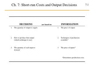
Ch. 7: Short-run Costs and Output Decisions. Costs in the Short Run. The short run is a period of time for which two conditions hold: The firm is operating with at least one factor of production being fixed. Firms can neither enter nor exit an industry.

E N D
Costs in the Short Run The short run is a period of time for which two conditions hold: • The firm is operating with at least one factor of production being fixed. • Firms can neither enter nor exit an industry. There are two types factors of production (inputs) in the short-run: fixed and variable two types of costs: fixed costs and variable costs. Fixed cost is any cost that does not depend on the firm’s level of output. These costs are incurred even if the firm is producing nothing. Variable cost is a cost that depends on the level of production chosen.
Costs in the Short Run Total Cost (TC) of Production is the sum of Total Fixed Costs (TFC) and Total Variable Costs (TVC): TC = TFC + TVC Total Fixed Costs (TFC): Firms have no control over fixed costs in the short run. For this reason, fixed costs are sometimes called sunk costs. Average fixed cost (AFC) is the total fixed cost (TFC) divided by the number of units of output (q)
q TFC AFC 0 55 1 55 55.00 2 55 27.50 3 55 18.33 4 55 13.75 5 55 11.00 6 55 9.17 7 55 7.86 8 55 6.88 9 55 6.11 10 55 5.50 Short-Run Fixed Cost (Total and Average) for Widget, Inc. AFC falls as output rises; a phenomenon sometimes called spreading overhead.
Total Variable Costs Total Variable Costs (TVC) depend on the level of production. The relationship should be positive: as the firm produces more output, total variable costs will increase. The question is how does it increase? Marginal cost (MC) is the increase in total cost that results from producing one more unit of output. Marginal cost reflects changes in variable costs. It measures the additional cost of inputs required to produce each successive unit of output. Because, by definition,
The Shape of the Marginal Cost Curve in the Short Run The fact that in the short run every firm is constrained by some fixed input(s) means that: • The firm has limited capacity to produce output • The firm faces diminishing marginal product for its variable inputs (Chapter 6) As a firm approaches that capacity, it becomes increasingly costly to produce successively higher levels of output. Example: From Ch. 6
The Shape of the Marginal Cost Curve in the Short Run Marginal costs ultimately increase with output in the short run.
Graphing Total Variable Costs and Marginal Costs: Widget, Inc. Total variable costs always increase with output. The marginal cost curve shows how total variable cost changes with single unit increases in total output. For output levels below q=3, TVC increases at a decreasing rate. For output levels above q=3, TVC increases at an increasing rate.
Graphing Total Variable Costs and Marginal Costs: The General Case $ • Total variable costs always increase with output. • In general, TVC might initially increase with q at a decreasing rate, but will eventually begin to increase with q at an increasing rate due to the law of diminishing marginal product (diminishing returns) TVC q qo $ per unit MC qo q
Average Variable Cost Average variable cost (AVC) is the total variable cost divided by the number of units of output. Marginal cost is the cost of one additional unit. Average variable cost is the average variable cost per unit of all the units being produced. Average variable cost follows marginal cost, but lags behind.
Relationship Between Average Variable Cost and Marginal Cost: Widget, Inc. MC AVC
Relationship Between Average Variable Cost and Marginal Cost: The General Case When marginal cost is below average cost, average cost is declining. This occurs for output levels below q1. When marginal cost is above average cost, average cost is increasing. This occurs for output levels greater than q1. Rising marginal cost intersects average variable cost at the minimum point of AVC. $ per unit MC AVC q qo q1 For output levels between qo and q1, MC is rising (diminishing returns set in) but MC is still less than AVC, so AVC continues to fall.
Total Costs: The General Case Adding TFC to TVC means adding the same amount of total fixed cost to every level of total variable cost. Thus, the total cost curve has the same shape as the total variable cost curve; it is simply higher by an amount equal to TFC. TC = TVC + TFC
Total Costs: Widget, Inc. The curvature pf TVC amd TC is not obvious in this graph, but an examination of the numbers shows us that rate of increase in total costs is initially decreasing and then begins to increase. TC TVC TFC
Average Total Cost: The General Case Average total cost (ATC) is total cost divided by the number of units of output (q). ATC = AFC + AVC but also: Because AFC falls with output, an ever-declining amount is added to AVC.
Relationship Between Average Total Cost and Marginal Cost: General Case • If marginal cost is below average total cost, average total cost will decline toward marginal cost. • If marginal cost is above average total cost, average total cost will increase. • Marginal cost intersects average total cost and average variable cost curves at their minimum points.
Interpreting the Numbers Pick an output level and examine the numbers: IF our widget manufacturer produces q = 4 units Total costs are TC = $160 where $55 of this cost is fixed and must be paid even if the firm produces q = 0 units; $105 are total variable costs: the cost of the variable inputs that were used to produce the 4 units of output. MC = $30 meaning the 4th unit increased total costs by $30. On the margin, the 4th unit incurred $30 in additional variable costs. ATC = $ 40 which is $ 40 per unit produced. On average each of the 4 units cost $ 40 to produce. AVC = $ 26.25 which is $ 26.25 per unit produced. On average, each of the 4 units incurred $26.25 in variable costs. AFC = $13.75 which is $ 13.75 per unit produced. On average, each of the 4 units incurred $13.75 in fixed costs.
Output Decisions: Revenues, Costs, and Profit Maximization In the short run, a competitive firm faces a demand curve that is simply a horizontal line at the market equilibrium price. The firm “looks” to the market to get the market price. Now it must decide what output level to offer for sale (its “quantity supplied”). Widget Firm Widget Market S d $70 $70 D Q q
Total Revenue (TR) andMarginal Revenue (MR) Total revenue (TR) is the total amount that a firm takes in from the sale of its output. TR = p * q Marginal revenue (MR) is the additional revenue that a firm takes in when it increases output by one additional unit. Because a perfectly competitive firm can all it wants to at the market price, P = MR. (Price and Marginal Revenue are equivalent concepts)
Comparing Costs and Revenues to Maximize Profit The Profit-Maximizing Rule: The profit-maximizing level of output (q*) for all firms is the output level where MR = MC. • The key idea is that firms will ↑ q long as MR > MC. But as q ↑, MC ↑ while MR stays flat. The firm will maximize profits at the output level q where MR = MC. Beyond this output level, the firm would not want to ↑ q because that would cause MC > MR and thus lower profits. • But, in perfect competition, MR≡P the profit-maximizing perfectly competitive firm will produce up to the point where the marginal cost of the last unit produced equals the price it receives from selling this last unit (q* is where P = MC)
Profit Analysis for Widget, Inc. Apply the profit-maximizing rule: find q* where P = MC. This occurs at q = 6. The profit levels for the various output levels are shown in the last column. It is true that q = 5 yields the same profit as q = 6. This does not invalidate the rule; the discrepancy is due to the “whole numbers” problem
Graph of Profit-Maximization Widget Market Widget Firm S MC ATC $70 d $70 AVC D q*=6 At any market price, the marginal cost curve shows the output level that maximizes profit. Thus, the marginal cost curve of a perfectly competitive profit-maximizing firm is the firm’s short-run supply curve with one caveat that we will study in the next chapter.