Download
1 / 25
250 likes | 389 Vues
Modeling study of the coastal upwelling system of the Monterey Bay area during 1999 and 2000. I. Shulman (1), J.D. Paduan (2), L. K. Rosenfeld (2), S. R. Ramp (2), J. C. Kindle (1). Naval Research Laboratory, Stennis Space Center, MS (2) Naval Postgraduate School, Monterey, CA. SUPPORT :

E N D
Modeling study of the coastal upwelling system of the Monterey Bay area during1999 and 2000. I. Shulman (1), J.D. Paduan (2), L. K. Rosenfeld (2), S. R. Ramp (2), J. C. Kindle (1) • Naval Research Laboratory, Stennis Space Center, MS • (2) Naval Postgraduate School, Monterey, CA SUPPORT: NOPP “Innovative Coastal-Ocean Observing Network (ICON)” ONR Ocean Modeling and Prediction ONR Biological and Chemical Oceanography
OUTLINE • Physical Model Configuration • Model Validation and Related Issues • Data Assimilation • Conclusions and Future Plans
Hierarchy of differentresolution models in the Pacific Ocean.Provides large-scale, basin-scale and small-scale view on the Monterey Bay circulation. Global (NLOM or NCOM) PWC (POM or NCOM)
ICON MODEL • Grid resolution ~ 1-4 km, 30 vertical • Open boundary conditions are derived from Pacific West Coast (PWC) NRL model (resolution ~10km). • Atmospheric forcing from NOGAPS and COAMPS predictions. • Assimilation of CODAR data. M2 M1 M3 M4
Observed and ICON model SSTsAugust 31, 1999 Santa Crus Pt. Sur
Impact of high-resolution wind forcing on ICON model predictions
ICON forced with 9km wind ( COAMPS) PWC forced with ~ 90km wind (NOGAPS)
ICON forced with 9km wind (COAMPS) PWC forced with 27km wind (COAMPS)
0.8C 0.1C Standard Deviation of SST. 4-6/99, energy at periods > 90 d removed NOGAPS (91km) COAMPS (9km) The model run with COAMPS 9km wind forcing better captured the influence of the complex coastline and topography structure. The model run with COAMPS 9km wind displayed more details and produced stronger headland effects. D. Blencoe, MS thesis
Coupling with larger-scale PWC modelComparison ADCP and model-predicted currentsat buoy M2 Magnitude of complex correlation Angular displacements
Impact of surface heat forcing on ICON model predictions. Observed and model predicted MLDs (m) 0.1 ˚C 0.2 ˚C 0.1 ˚C 0.2 ˚C
Offshore core of the California current California Undercurrent
California UndercurrentRAFOS floats vs ICON model currents, 300m
Conclusion • With high-resolution atmospheric forcing the ICON model captures “the essence” but not the “details”of observed variability. • Data Assimilation (“blending” of observations and model predictions) is needed
HIGH FREQUENCY RADAR (CODAR) DATA ASSIMILATION IN THE MONTEREY BAY.
APPROACH Figure 4. Alongshore component of wind at the M1 mooring and the mode 1 amplitude for the radar-derived (CODAR) surface velocity fields as a scatter plot (left panel) and versus time (right panel). Methods of using HF radar data to provide corrections to the model wind forcing are investigated. Inadequate knowledge of the wind stress is probably a significant source of error in the model solutions.
Figure 6. CODAR data footprints (dots) and locations of M1 and M2 moorings
Magnitudes of complex correlation (a) and angular displacements (b) between model-predicted currents and those observed at M2.
Map of complex-correlation magnitudes between observed currents at M2 and HF radar-derived surface currents (upper level in each panel) or model-predicted currents at various depths. No assim. With assim.
Map of complex-correlation magnitudes between observed currents at M1 and HF radar-derived surface currents (upper level in each panel) or model-predicted currents at various depths. With assim. No assim.
Div M ICON forced with ~90km wind (NOGAPS)
Bioluminescence maximums at 242d and 245th days are located in the frontal areas representing a strong reversal of flow direction. AA BB 242d day 245th day Bioluminescence Along-shore model velocities Section AA Section BB
FUTURE • Use of circulation model for optimal and adaptive sampling • Bio-optical and physical modeling • Data Assimilation: CODAR, SSTs, glider and mooring data, estimation and modeling covariances.