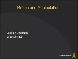
Motion and Manipulation
Motion and Manipulation. Collision Detection. 1. Collision Detection. Sampling-based path planning: check if a simple path between two neighboring configurations is collision-free Detect collision of objects that move under the influence of physics laws are controlled by a user

Motion and Manipulation
E N D
Presentation Transcript
Motion and Manipulation Collision Detection 1
Collision Detection Sampling-based path planning: check if a simple path between two neighboring configurations is collision-free Detect collision of objects that move under the influence of physics laws are controlled by a user Collisions often require actions: compute deformation, change direction and magnitude speed 2
Standard Approach t := 0 while not ready do compute placements of objects at t + ∆t check for intersections of objects at these placements, and perform action if necessary t := t + ∆t 3
Collision or Interference Checking t := 0 while not ready do compute placements of objects at t + ∆t check for intersections of objects at these placements, and perform action if necessary t := t + ∆t Choice of ∆t is crucial! 4
Time Step ∆t too large: danger of undetected collisions ∆t too small: excessive computation time t + ∆t t 5
Expensive Alternative Use sweep volumes, or add time dimension Disadvantages complex shapes, expensive computation motion must be known beforehand t t y t + ∆t x 6
Interference Checking Given: set P of n primitives (e.g. triangles, lines) or objects (e.g. convex polygons or polytopes) Approach Filtering step, or broad phase: smart selection (using a data structure) of pairs of primitives/objects that may intersect Refinement step, or narrow phase: actual intersection check of candidate pairs resulting from filtering step 7
Refinement Step • Primitive-primitive collisions • Object-object collisions
Refinement Step: Primitives (Fast) intersection tests for primitives are non-trivial Test: does tetrahedron A intersect tetrahedron B? 9
Refinement Step Test: does tetrahedron A intersect tetrahedron B? Solution: edge of A intersects triangular facet of B, or edge of B intersects triangular facet of A, or vertex of A lies inside B, or vertex of B lies inside A 10
Refinement Step Test: does point p lie inside simple polyhedron A? 11
Refinement Step Test: does point p lie inside simple polyhedron A? Solution: count number of intersections of a half-line emanating from p with boundary facets of A if odd: p lies inside A if even: p is not in A beware: degenerate cases! 12
Refinement Step Test: does segment pq intersect triangle abc? c q a b p 13
Refinement Step Test: does segment pq intersect triangle abc? Solution: p and q lie on opposite sides of plane through a, b, and c and q and c lie on same side of plane through a, b, and p and q and b lie on same side of plane through a, c, and p and q and a lie on same side of plane through b, c, and p c q a b p 14
Refinement Step: Objects • The distance between two non-intersecting objects is the minimum distance between a point in the first object and a point in the second object (or the minimum distance these objects need to translate to become intersecting) • The penetration depth of two intersecting objects is the minimum distance these objects need to translate to become disjoint
Refinement Step: Objects • The Gilbert-Johnson-Kheerti (GJK) algorithm computes the distance or penetration depth for two convex objects A and B, which equals the (shortest) distance from the origin to the Minkowski sum of A and –B (or of B and –A) • The Chung-Wang (CW) algorithm is an improvement of GJK for a specific class of convex objects
Separating Axis Theorem • A separating axis of two disjoint objects A and B is a vector v such that the projections of A and B onto v do not overlap • For any pair of nonintersecting polytopes, there exists a separating axis that is orthogonal to a facet of either polytope, or orthogonal to an edge from each polytope
Separating Axis Tests • This means that for a pair of polytopes with f1 and f2 facet orientations respectively and e1 and e2 edge orientations respectively, we need to test f1+f2+e1e2 axes for separation • Number of tests is high; examples (in 3D): • triangle – triangle 11 tests • triangle – box 13 tests • box – box 15 tests
Terminology: Separating Plane • A strongly separating plane strictly leaves two objects on opposite sides; strongly separating planes are very hard to find • A weakly separating plane leaves two objects on opposite sides (probably touching them)
Terminology: Support Mapping • Gives (an) extreme point SC(d) in C in any direction d
Terminology: Simplex 0-simplex 1-simplex 2-simplex 3-simplex simplex
Terminology: Convex Hull Point set C Convex hull, CH(C)
GJK Algorithm • Initialize the simplex set Q with up to d+1 points from C (in d dimensions) • Compute point P of minimum norm in CH(Q) • If P is the origin, exit; return 0 • Reduce Q to the smallest subset Q’ of Q, such that P in CH(Q’) • Let V=SC(–P) be a supporting point in direction –P • If V no more extreme in direction –P than P itself, exit; return ||P|| • Add V to Q. Go to step 2
GJK example 1(10) INPUT: Convex polytope C given as the convex hull of a set of points
GJK example 2(10) • Initialize the simplex set Q with up to d+1 points from C (in d dimensions)
GJK example 3(10) • Compute point P of minimum norm in CH(Q)
GJK example 4(10) • If P is the origin, exit; return 0 • Reduce Q to the smallest subset Q’ of Q, such that P in CH(Q’)
GJK example 5(10) • Let V=SC(–P) be a supporting point in direction –P
GJK example 6(10) • If V no more extreme in direction –P than P itself, exit; return ||P|| • Add V to Q. Go to step 2
GJK example 7(10) • Compute point P of minimum norm in CH(Q)
GJK example 8(10) • If P is the origin, exit; return 0 • Reduce Q to the smallest subset Q’ of Q, such that P in CH(Q’)
GJK example 9(10) • Let V=SC(–P) be a supporting point in direction –P
GJK example 10(10) • If V no more extreme in direction –P than P itself, exit; return ||P|| DONE!
Filtering Step Prevent testing all pairs of primitives for intersection, but use data structure to select a (preferably small) set of candidates Approaches Space partitioning Model partitioning 34
Space Partitioning Decompose space into cells Store references to intersecting primitives with each cell cell x cell x cell y cell y 35
Space Partitioning Idea: only test pairs of primitives that intersect the same cell (and at least one of the primitives is moving) Issue: store moving objects in data structure or not (and instead just query with them)? Storing moving objects requires updates of the data structure 36
Query with Moving Object cell x cell x cell y cell y 37
Voxel Grid Use regular grid for subdivision of space j i • Subdivision is stored implicitly • Fast access of cells 38
Voxel Grid Cluttered scenes • Distribution is not taken into account 39
Voxel Grid Differently-sized objects Voxel grids work well for roughly uniformly-distributed and equally-sized objects 40
Quadtree (or Octree) Take distribution into account by appropriately varying cell size Square/cubic cells only Top-down decomposition: subdivide a cell only if the number of objects intersecting it is (too) large 41
Quadtree Build Quadtree (set P, square σ): if P and σ satisfy stop criterion then create leaf for σ and store references to elements of P else split σ into four quadrants σ1…σ4 determine subsets Pi of P of objects intersecting σi create internal node ν, with the trees resulting from recursively running Build Quadtree (Pi , σi) for 1≤i ≤4 as its children 42
Quadtree 43
Quadtree More adaptive than voxel grids • Extra overhead: tree structure • Slower access of cells Still many empty cells in case of uneven object distribution 44
Kd Tree More freedom in subdivision: splits by means of axis-parallel line Horizontal or vertical: alternatingly longest side first Location: bisecting vertices bisecting centroids 45
Kd Tree l1 l2 l3 l2 l3 l1 46
Kd Tree Problematic scene 47
BSP Tree Even more freedom in subdivision: splits by means of any line 48
Space Partitioning General disadvantage: multiple references to the same object (due to that object intersecting multiple cells): requiring extra memory leading to multiple intersection tests for the same pair during an interference query 49
Model Partitioning Strategies use bounding volumes Bounding volume of an object is a primitive shape that encloses the object Idea: if a query object does not intersect a bounding volume it does also not intersect the enclosed object 50