STATISTICAL ANALYSIS AND SOURCE LOCALISATION
This comprehensive guide explores statistical analysis and source localization techniques for EEG and MEG data, tailored for beginners. It covers essential concepts such as signal sources, dipoles, preprocessing, and experimental design. The importance of statistical significance and effective correction of multiple tests are emphasized. Learn about various analysis methods, including sensor-level analysis and time-frequency analysis, as well as the challenges of source localization, including the ill-posed inverse problem and Bayesian approaches. Ideal for students and researchers in neuroimaging.


STATISTICAL ANALYSIS AND SOURCE LOCALISATION
E N D
Presentation Transcript
STATISTICAL ANALYSIS AND SOURCE LOCALISATION METHODS FOR DUMMIES 2012-2013 ANADUAKA, CHISOM KRISHNA, LILA UNIVERSITY COLLEGE LONDON
M/EEG SO FAR • Source of Signal • Dipoles • Preprocessing and Experimental design
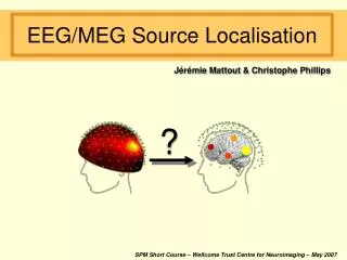
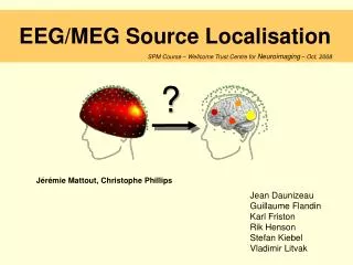
E/MEG SIGNAL Source Reconstruction Statistical Analysis
How does it work? Statistical analysis 1. Sensor level analysis in SPM 2. Scalp vs. Time Images 3. Time-frequency analysis
Neuroimaging produces continuous data e.g. EEG/MEG data. • Time varying modulation of EEG/MEG signal at each electrode or sensor. • Statistical significance of condition specific effects. • Effective correction of number of tests required- FWER.
Steps in SPM • Data transformed to image files (NifTI) • Between subject analysis as in “2nd level for fMRI” • Within subject possible • Generate scalp map/time frame using 2D sensor layout and linear interpolation btw sensors (64 pixels each spatial direction suggested)
Space-space-time maps SPM Sensor level analysis a EVOKED SCALP RESPONSE SLOW EVOLUTION IN TIME In
Sensor Level Analysis • This is used to identify pre-stimulus time or frequency windows. • Using standard SPM procedures(topological inference) applied to electromagnetic data; features are organised into images. Raw contrast time frequency maps SPM Smoothing Kernel
Topological inference • Done when location of evoked/induced responses is unknown • Increased sensitivity provided smoothed data • Vs Bonferroni: acknowledges non-independent neighbours • ASSUMPTION Irrespective of underlying geometry or data support, topological behaviour is invariant.
Time vs. Frequency data • Time-frequency data: Decrease from 4D to 3D or 2D time-frequency (better for SPM). • Data features: Frequency-Power or Energy(Amplitudes) of signal. • Reduces multiple comparison problems by averaging the data over pre-specified sensors and time bins of interest.
Averaging Averaging over time/frequency • Important: requires prior knowledge of time window of interest • Well characterised ERP→2D image + spatial dimensions • E.g. Scalp vs. time or Scalp vs. Frequency
Smoothing step • Smoothing: prior to 2nd level/group analysis -multi dimensional convolution with Gaussian kernel. Multi-dimensional convolution with Gaussian kernel • Important to accommodate spatial/temporal variability over subjects and ensure images conform to assumptions.
Source localisation • Source of signal difficult to obtain • Ill-posed inverse problem (infers brain activity from scalp data): Any field potential vector can be explained with an infinite number of possible dipole combinations. • Absence of constraints No UNIQUE solution • Need for Source Localisation/Reconstruction/Analysis
NO CORRECT ANSWER; AIM IS TO GET A CLOSE ENOUGH APPROXIMATION….
Forward/Inverse problems Forward model: • Gives information about Physical and Geometric head properties. • Important for modeling propagation of electromagnetic field sources. • Approximation of data from Brain to Scalp. Backward model/Inverse Problem: • Scalp data to Brain • Source localization in SPM solves the Inverse problem.
Forward/Inverse problems FORWARD PROBLEM INVERSE PROBLEM
Forward/Inverse problems Head model: conductivity layout Source model: current dipoles Solutions are mathematically derived.
Source reconstruction • Source space modeling • Data co-registration • Forward computation • Inverse reconstruction • Summarise reconstructed response as image FORWARD MODEL
Data co-registration Rotation • Rigid-body transformation matrices • Fiducial matched to MRI applied to sensor positions • Surface matching: between head shape in MEEG and MRI-derived scalp tessellations. It is important to specify MRI points corresponding to fiducials whilst ensuring no shift Transformation
Data Co-registration “Normal” cortical template mesh (8196 vertices), left view Example of co-registration display (appears after the co-registration step has been completed)
Forward computation • Compute effects on sensors for each dipole • N x M matrix • Single shell model recommended for MEG, BEM(Boundary Element Model) for EEG. No of sensors No of mesh vertices
Distributed source reconstruction • 3D • Using Cortical mesh Forward model parameterisation • Allows consideration of multiple sources simultaneously. • Individual meshes created based on subject’s structural MR scan–apply inverse of spatial deformation
Y = kJ + E Data gain matrix noise/error • Estimate J (dipole amplitudes/strength) • Solve linear optimisation problem to determine Y • Reconstructs later ERP components Problem • Fewer sensors than sources • needs constraints
Constraints • Every constraint can provide different solutions • Bayesian model tries to provide optimal solution given all available constraints POSSIBILITIES • IID- Summation of power across all sources • COH- adjacent sources should be added • MSP- data is a combination of different patches Sometimes MSP may not work.
Bayesian principle • Use probabilities to formalize complex models to incorporate prior knowledge and deal with randomness, uncertainty or incomplete observations. • Global strategy for multiple prior-based regularization of M/EEG source reconstruction. • Can reproduce a variety of standard constraints of the sort associated with minimum norm or LORETA algorithms. • Test hypothesis on both parameters and models
Summarise Reconstructed Data • Summarise reconstructed data as an image • Summary statistics image created in terms of measures of parameter/activity estimated over time and frequency(CONTRASTS) • Images normalised to reduce subject variance • The resulting images can enter standard SPM statistical pipeline (via ‘Specify 2nd level’ button).
Equivalent Current Dipole (ECD) • Small number of parameters compared to amount of data • Prior information required • MEG data Y=f(a)+e • Reconstructs Subcortical data • Reconstructs early components ERPs (Event related potentials) • Requires estimate of dipole direction Problem Non-linear optimisation
Dipole Fitting Estimated data Estimated Positions Measured data
Variationalbayesian- ECD • Priors for source locations can be specified. • Estimates expected source location and its conditional variance. • Model comparison can be used to compare models with different number of sources and different source locations.
VB-ECD • ASSUMPTIONS • Only few sources are simultaneously active • Sources are focal • Independent and identical normal distribution for errors • Iterative scheme which estimates posterior distribution of parameters • Number of ECDs must not exceed no of channels÷6 • Non-linear form- optimise dipole parameters given observed potentials • takes into account model complexity • Prepare head model as for 3D
Extras • Rendering interface: extra features e.g. videos • Group inversion: for multiple datasets • Batching source reconstruction: different contrasts for the same inversion
IN SPM • Activate SPM for M/EEG: type spmeegon MATLAB command line enter • GUI INTERFACE BETTER FOR NEW USERS LIKE ME!!!!! Instructions are clearly outlined.
Forward computation inversion 2
REFERENCES • SPM Course – May 2012 – London • SPM-M/EEG Course Lyon, April 2012 • TolgaEsatOzkurt-High Temporal Resolution brain Imaging with EEG/MEG Lecture 10: Statistics for M/EEG data • James Kilner and Karl Friston. 2010.Topological Inference for EEG and MEG. Annals of Applied Statistics Vol 4:3 pp 1272-1290 • Vladimir Litvak et al. 2011. EEG and MEG data analysis in SPM 8. Computational Intelligence and Neuroscience Vol 2011 • MFD 2011/12