Download
1 / 77
770 likes | 901 Vues
CPSC 461 Clustering. Dr. Marina Gavrilova Associate Professor, Department of Computer Science, University of Calgary, Calgary, Alberta, Canada. Lecture outline. Clustering in research Clustering in data mining Clustering methods Clustering applications in path planning Summary.

E N D
CPSC 461 Clustering Dr. Marina Gavrilova Associate Professor,Department of Computer Science, University of Calgary, Calgary, Alberta, Canada.
Lecture outline • Clustering in research • Clustering in data mining • Clustering methods • Clustering applications in path planning • Summary
The Problem • Given two locations A and B and the geographical features of the underlying terrain, what is the optimal route for a mobile agent between these two locations? • When the nature of the terrain is allowed to vary, the robot has to make a decision which path is the most suitable based on the set of priorities. • We concentrate on marine applications, where robot is conceived as a ship sailing from one port to another. The decision making process can become very complex and combines AI, uncertainty theory and multi-varied logic with temporal-spatial data representation. • The problem arises in such areas as Robotics, Risk Planning, Route Scheduling, Navigation, and Processes Modeling. The risk areas are defined by cluster analysis performed on the incident database of the Maritime Activity and Risk Investigation System (MARIS).
The Geometry-based approach • Design of a new topology-based space partitioning (Delaunay triangulation) based clustering method to identify complicated cluster arrangements. • Development of an efficient Delaunay triangulation and visibility graph based method for determining clearance-based shortest path between source and destination in the presence of simple, disjoint, polygonal obstacles. • Introduction of a new method for determining optimal path in a weighted planar subdivision representing a varied terrain.
System Flowchart Incident locations from MARIS database Cluster analysis Polygon Fitting Sea-ice layer High risk areas Optimal path planning Optimal path Landmass layer
Marine Risk Analysis • Identification of high-risk areas in the sea based on incident and traffic data from the Maritime Activity and Risk Investigation System (MARIS), maintained primarily by the University of Halifax. Incident data Marine Route Planning Clustering Algorithm High-risk Areas Location of SAR Bases Ship route intersection data
Definition of Clustering • Clustering is the unsupervised classification of patterns (observations, data items or feature vectors) into groups (clusters). – A.K. Jain, M. N. Murty, P. J. Flynn, Data Clustering: A Review Clustering a collection of points
Clustering – desired properties • Linear increase in processing time with increase in size of dataset (scalability). • Ability to detect clusters of different shapes and densities. • Minimal number of input parameters. • Robust with regard to noise. • Insensitive to data input order. • Portable to higher dimensions. Osmar R. Zaΐane, Andrew Foss, Chi-Hoon Lee, Weinan Wang, “On Data Clustering Analysis: Scalability, Constraints and Validation”, Advances in Knowledge Discovery and Data Mining, Springer-Verlag, 2002.
Clustering in data mining: Unsupervised Learning • Given: • Data Set D (training set) • Similarity/distance metric/information • Find: • Partitioning of data • Groups of similar/close items
Similarity? • Groups of similar customers • Similar demographics • Similar buying behavior • Similar health • Similar products • Similar cost • Similar function • Similar store • … • Similarity usually is domain/problem specific
Distance Between Records • d-dim vector space representation and distance metric r1: 57,M,195,0,125,95,39,25,0,1,0,0,0,1,0,0,0,0,0,0,1,1,0,0,0,0,0,0,0,0 r2: 78,M,160,1,130,100,37,40,1,0,0,0,1,0,1,1,1,0,0,0,0,0,0,0,0,0,0,0,0,0 ... rN: 18,M,165,0,110,80,41,30,0,0,0,0,1,0,0,0,0,0,0,0,0,0,0,0,0,0,0,0,0,0 Distance (r1,r2) = ??? • Pair wise distances between points (no d-dim space) • Similarity/dissimilarity matrix(upper or lower diagonal) • Distance: 0 = near, ∞ = far • Similarity: 0 = far, ∞ = near -- 1 2 3 4 5 6 7 8 9 10 1 - d d d d d d d d d 2 - d d d d d d d d 3 - d d d d d d d 4 - d d d d d d 5 - d d d d d 6 - d d d d 7 - d d d 8 - d d 9 - d
Properties of Distances: Metric Spaces • A metric space is a set S with a global distance function d. For every two points x, y in S, the distance d(x,y) is a nonnegative real number. • A metric space must also satisfy • d(x,y) = 0 iff x = y • d(x,y) = d(y,x) (symmetry) • d(x,y) + d(y,z) >= d(x,z) (triangle inequality)
Minkowski Distance (Lp Norm) • Consider two records x=(x1,…,xd), y=(y1,…,yd): Special cases: • p=1: Manhattan distance • p=2: Euclidean distance
Only Binary Variables 2x2 Table: • Simple matching coefficient:(symmetric) • Jaccard coefficient:(asymmetric)
Nominal and Ordinal Variables • Nominal: Count number of matching variables • m: # of matches, d: total # of variables • Ordinal: Bucketize and transform to numerical: • Consider record x with value xi for ith attribute of record x; new value xi’:
Mixtures of Variables • Weigh each variable differently • Can take “importance” of variable into account (although usually hard to quantify in practice)
Clustering: Informal Problem Definition Input: • A data set of N records each given as a d-dimensional data feature vector. Output: • Determine a natural, useful “partitioning” of the data set into a number of (k) clusters and noise such that we have: • High similarity of records within each cluster (intra-cluster similarity) • Low similarity of records between clusters (inter-cluster similarity)
Types of Clustering • Hard Clustering: • Each object is in one and only one cluster • Soft Clustering: • Each object has a probability of being in each cluster
Approaches to HARD clustering • Hierarchical clustering (Chameleon, 1999) • Density-based clustering (DBScan, 1996) • Grid-based clustering (Clique, 1998) • Model-based clustering (Vladimir, Poss, 1996) • Partition-based clustering (Greedy Elimination Method, 2004) • Graph-based clustering (Autoclust, 2000)
Hierarchical Clustering • Creates a tree structure to determine the clusters in a dataset (top-down or bottom-up). Bottom-up: consider each data element as a separate cluster and then progressively merge clusters based on similarity until some termination condition is reached (agglomerative). Top-down: consider all data elements as a single cluster and then progressively divides a cluster into parts (divisive). • Hierarchical clustering does not scale well and the computational complexity is very high (CHAMELION). The termination point for division or merging for divisive and agglomerative clustering respectively is extremely difficult to determine accurately.
Density-based clustering • In density-based clustering, regions with sufficiently high data densities are considered as clusters. It is fast but it is difficult to define parameters such as epsilon-neighborhood or minimum number of points in such neighborhoods to be considered a cluster. • These values are directly related to the resolution of the data. If we simply increase the resolution (i.e. scale up the data), the same parameters no longer produce the desired result. • Advanced methods such as TURN consider the optimal resolution out of a number of resolutions and are able to detect complicated cluster arrangements but at the cost of increased processing time.
Grid-based clustering • Grid-based clustering performs clustering on cells that discretize the cluster space. Because of this discretization, clustering errors necessarily creep in. • The clustering results are heavily dependent on the grid resolution. Determining an appropriate grid resolution for a dataset is not a trivial task. If the grid is coarse, the run-time is lower but the accuracy of the result is questionable. If the grid is too fine, the run-time increases dramatically. Overall, the method is unsuitable for spatial datasets.
Model-based clustering • In model-based clustering, the assumption is that a mixture of underlying probability distributions generates the data and each component represents a different cluster . It tries to optimize the fit between the data and the model. Traditional approaches involve obtaining (iteratively) a maximum likelihood estimate of the parameter vectors of the component densities. Underfitting (not enough groups to represent the data) and overfitting (too many groups in parts of the data) are common problems, in addition to excessive computational requirements. • Deriving optimal partitions from these models is very difficult . Also, fitting a static model to the data often fails to capture a cluster's inherent characteristics. These algorithms break down when the data contains clusters of diverse shapes, densities and sizes.
Partition based clustering • Place K points into the space represented by the data points that are being clustered. These points represent initial group centroids. • Partition the data points such that each data point is assigned to the centroid closest to it. • When all data points have been assigned, recalculate the positions of the K centroids. • Repeat Steps 2 and 3 until the centroids no longer move.
K-Means Clustering Algorithm Initialize k cluster centers Do Assignment step: Assign each data point to its closest cluster center Re-estimation step: Re-compute cluster centers While (there are still changes in the cluster centers)
K-Means: Summary • Advantages: • Good for exploratory data analysis • Works well for low-dimensional data • Reasonably scalable • Disadvantages • Hard to choose k • Often clusters are non-spherical
Disadvantages • Number of clusters have to be prespecified. • Clustering result is sensitive to initial positioning of cluster centroids. • Able to detect clusters of convex shape only. • Clustering result is markedly different from human perception of clusters. Greedy Elimination Method (K = 5)
Recent Papers Z.S.H. Chan, N. Kasabov: “Efficient global clustering using the Greedy Elimination Method”, Electronics Letters, 40(25), 2004. Aristidis Likas, Nikos Vlassis, Jakob J. Verbeek: “The global k-means clustering algorithm”, Pattern Recognition, 36(2), 2003. Global K-Means (K = 5)
Summary of shortcomings of existing methods • Able to detect only convex clusters. • Require prior information about dataset. • Too many parameters to tune. • Inability to detect elongated clusters or complicated arrangements such as cluster within cluster, clusters connected by bridges or sparse clusters in presence of dense ones. • Not robust in presence of noise. • Not practical on large datasets.
Graph-based clustering – a good approach • The graph-based clustering algorithms based on the triangulation approach have proved to be successful. However, most algorithms based on the triangulation derive clusters by removing edges from the triangulation that are longer than a threshold (Eldershaw,Kang,Imiya). But distance alone cannot be used in separating clusters. The technique succeeds only when the intra-cluster distance is sufficiently high. It fails in case of closely lying high density clusters or clusters connected by bridges. • We utilize a number of unique properties of Delaunay triangulation , as it is an ideal data structure for preserving proximity information and effectively eradicates the problem of representing spatial adjacency using the traditional line-intersection model . It can be constructed in O(nlogn) time and has only O(n) edges.
Triangulation based clustering • Construct the Delaunay triangulation of the dataset. • Remove edges based on certain criteria with connected components eventually forming clusters. • Vladimir Estivill-Castro, Ickjai Lee, “AUTOCLUST: Automatic Clustering via Boundary Extraction for Mining Massive Point-Data Sets”, Fifth International Conference on Geocomputation, 2000. • G. Papari, N. Petkov, “Algorithm That Mimics Human Perceptual Grouping of Dot Patterns”, Lecture Notes in Computer Science, 3704, 2005, pp. 497-506. • Vladimir Estivill-Castro, Ickjai Lee, “AMOEBA: Hierarchical clustering based on spatial proximity using Delaunay Diagram”, 9th International Symposium on Spatial Data handling, 2000. Sparse graph Connected components
Disadvantages • The use of global density measures such as mean edge length is misleading and often precludes the identification of sparse clusters in presence of dense ones. • The decision of whether to remove an edge or not is usually a costly operation. Also, deletion of edges may result in loss of topology information required for identification of later clusters. As a result, algorithms often have to recuperate some of the lost edges later on.
CRYSTAL - Description • Initialization phase: Generates the Voronoi diagram of the data points and sorts them in increasing order of the area of their Voronoi cells. This ensures that clustering starts with the densest clusters. • Grow cluster phase:Scans the sorted vertex list L and for each vertex Vi € L not yet visited, attempts to grow a cluster. The Delaunay triangulation is utilized as the underlying graph on which a breadth-first search is carried out. The cluster growth stops at a point identified as a boundary point but continues from other non-boundary points. Several criteria are employed to effectively determine the cluster boundary. • Noise removal phase: Identifies noise as sparse clusters or clusters that have very few elements. They are removed at this stage.
Merits of CRYSTAL • The growth model adopted for cluster growth allows spontaneous detection of elongated and complicated cluster shapes. • The algorithm avoids the use of global parameters and makes no assumptions about the data. • The clusters fail to grow from noise points or outliers. Thus noise can be easily eliminated without any additional processing overhead. • The algorithm works very fast in practice as the growth model ensures that identification of different cases like cluster within cluster or clusters connected by bridges do not require any additional processing logic and are handled spontaneously. • It requires no input parameter from user and the clustering output closely resembles human perception of clusters.
CRYSTAL – Geometric Algorithms • Triangulation phase: Forms the Delaunay Triangulation of the data points and sorts the vertices in the order of increasing average length of incident edges. This ensures that, in general, denser clusters are identified before sparser ones. • Grow cluster phase: Scans the sorted vertex list and grows clusters from the vertices in that order, first encompassing first order neighbors, then second order neighbors and so on. The growth stops when the boundary of the cluster is determined. A sweep operation adds any vertices to the cluster that may have been left out. • Noise removal phase: The algorithm identifies noise as sparse clusters. They can be easily eliminated by removing clusters which are very small in size or which have a very low spatial density.
Average cluster edge length = Average of the length of edges incident on the vertex d = Edge Length between the two vertices (d) d2 d1 = (d1 + d2) / 2 In general, (Sum of edge lengths) / (Number of elements in cluster – 1)
Detecting a cluster boundary Boundary vertex Mean of incident edge lengths of Vi > 1.6 * Average cluster edge length? Boundary vertex Vertex Vi Inner point of the cluster
Grow cluster phase Enqueue( Q, vk ) C← vk tot_dist ← 0 AvgadjEdgeLen( vi ) – Average of the length of edges incident on a vertex vi avg ← AvgadjEdgeLen( vk ) d ← Head( Q ) L ← 1st-order neighbors of d sorted by edge length For all LiєL do C← CU Li tot_dist ← tot_dist + EdgeLen( d, Li ) avg ← tot_dist / (Size( C ) - 1) If Not a boundary vertex and Not connected to a boundary vertex then Enqueue( Q, Li ) End If End For EdgeLen( vi ,vj ) – Euclidean distance between vertices vi and vj Dequeue(Q) Q = Φ ? Y Perform sweep and consider next vertex N
Sweep • The average cluster edge length towards the end of Grow Cluster phase better represents the local density than at the starting phase of cluster growth. • This operation ensures that any data points that were left out at the initial stages of the cluster growth are put back into the cluster. • Scan the vertices added to cluster. • For each vertex, inspect if there are any 1st order neighbors for which edge length < 1.6 * average cluster edge length. If so, add that vertex to the cluster and update the average cluster edge length. Description:
Boundary detection A vertex is considered to be a boundary vertex of the cluster if any one of the following is true: • Voronoi cell area of the vertex in the Voronoi diagram is > Th * {average Voronoi cell area of cluster} • The maximum of the Voronoi cell areas of the neighbors of the vertex (including itself) > Th * {average Voronoi cell area of cluster} • The vertex is connected to another vertex in the Delaunay Triangulation which is already present in the cluster so that the edge length is > Th * {average cluster edge length} The value of Th is empirically determined.
Sample output Original dataset (n = 8,000) CRYSTAL output (Th = 2.4)
Comparison Reduced Delaunay Graph from 1 Discontinuity CRYSTAL output 1G. Papari, N. Petkov, “Algorithm That Mimics Human Perceptual Grouping of Dot Patterns”, Lecture Notes in Computer Science, 3704, 2005, pp. 497-506.
Comparison CRYSTAL G. Papari, N. Petkov, “Algorithm That Mimics Human Perceptual Grouping of Dot Patterns”, Lecture Notes in Computer Science, 3704, 2005, pp. 497-506.
A E F B G C Clustering results on t7.10k dataset Osmar R. Zaΐane, Andrew Foss, Chi-Hoon Lee, Weinan Wang, “On Data Clustering Analysis: Scalability, Constraints and Validation” H D
CRYSTAL output t7.10k dataset (9 visible clusters, n = 10,000)
CRYSTAL output CRYSTAL on t7.10k dataset (Г = 1.8)
More examples Original dataset Crystal output (Th = 2.5) Original dataset Crystal output (Th = 2.4)