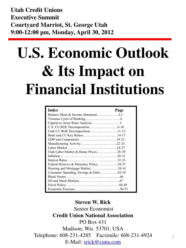
Utah Credit Unions Executive Summit Courtyard Marriot, St. George Utah

1. Utah Credit Unions Executive Summit Courtyard Marriot, St. George Utah 9:00-12:00 pm, Monday, April 30, 2012 U.S. Economic Outlook & Its Impact on Financial Institutions Steven W. Rick Senior Economist Credit Union National Association PO Box 431 Madison, Wis. 53701, USA Telephone: 608-231-4285 Facsimile: 608-231-4924 E-Mail: srick@cuna.com Index Page Balance Sheet & Income Statement………...……..2,3 Virtuous Cycle of Banking………………………….4 Capital-to-Asset Ratio Analysis…………………….5 U.S. CU ROE Decomposition……………….........6-10 Utah CU ROE Decomposition……………………11-13 Bank and CU Key Ratios………………….….......14-17 GDP and Components……………………………18-21 Manufacturing Activity…………………………..22-23 Labor Market ………………………………..…...24-27 Utah Labor Market & Home Prices………………28-29 Inflation…………………………………….……..30-31 Interest Rates………………………………..…….32-33 Federal Reserve & Monetary Policy………..…….34-37 Housing and Mortgage Market……………..……..38-41 Consumer Spending, Savings & Debt………..…...42-45 Black Swans………………………………………...46 Oil and Stock Markets……………………….……..47 Fiscal Policy………………………………….…….48-49 Economic Forecast………………………………….50-51

2. Deposit Factors: Economic uncertainty and members’ preference for liquid funds will buoy deposits. Large interest rate differentials between loans and savings will encourage households to pay down debt rather than save any surplus funds. Households using existing savings balances to pay down debt will reduce size of balance sheet. Rising oil prices will reduce savings balances. Inflation rates higher than deposit rates will produce negative returns on savings deposits. Large federal deficits may lead to expectations of higher future taxes fostering additional savings growth today. The national savings rate is back to the level in the late 1990s. Falling home prices will encourage thrift. Investment Factors: Federal Reserve announced that economic conditions “are likely to warrant exceptionally low levels for the federal funds rate at least through late 2014 is forcing a reevaluation of the duration of investments. Rising loan growth will reduce investment portfolio growth in 2012. Financial institutions are sitting on record levels of excess reserves ($1.6 trillion) earning 0.25%. Excess liquidity is punishing earnings with short-term investment yields lower than deposit interest rates. CU Balance Sheet (% of 2010 Assets) Assets Liabilities + NW Investments (34%) Deposits (86%) Loans (62%)Net Worth (10%) Annual Growth Rates Annual Growth Rates Annual Growth Rates Annual Growth Rates Loan Factors: Economic recovery and accompanying job growth will encourage borrowing in 2012. Rising consumer confidence will encourage spending. Rising stock prices will produce a “wealth effect” fostering increased consumption. Household s have accelerated loan payments and payoffs which is outpacing originations and reducing loan balances. But deleveraging should fade in 2012. Low spending in 2009-2011 has created much pent-up demand for durable goods. Auto loans, credit card loans and purchase mortgage loans will be strong growth areas. The recession has created a large pool of potential borrowers with sub-prime credit scores. Rising auto sales may reduce 0% financing offers. Udall-Snow Small Business Lending Enhancement Act is moving in Congress to raise the business loan lending cap from 12.25% to 27.5% of assets for CUs. Net Worth Factors: Rising net income in 2012. Capital contributions will outpace asset growth raising net worth-to-asset ratios. CUs are slowing deposit and asset growth to maintain or boost capital-to-asset ratios. BASEL III will be an impetus for Congress and NCUA for capital reform. Alternative capital (subordinated debt) is a top CU legislative priority.

3. The Federal Reserve’s QE-2 program (print money to buy bonds) and Operation Twist will keep long-term interest rates low through 2013. Banks/CUs are weighing the marginal risk (credit/interest rate) versus marginal return (additional YOA) of alternative assets to boost NIMs. Repricing of maturing loans will lower YOAs Rising loan growth will raise YOAs. Rising short-term interest rates in 2014 will raise yields on short-term investments. Yield on Assets - Cost of Funds = NIM + Fee/Other Income - Operating Expenses - Provision for loan losses = Net Income Rising short-term interest rates in 2014 will increase COFs. Continued repricing of maturing CDs is lowering COFs today. Excess liquidity will allow Bank/CU deposit rates to lag increases in market rates in 2014. Ultra-low market interest rates are preventing the pricing of deposits below market, reducing earnings opportunities . NIM expected to rise in 2015 as YOA rise faster than COFs. A flatter yield curve in 2012 will put downward pressure on NIMs by making ST borrowing and LT lending less lucrative. Banks/CUs are reevaluating their “GAP” strategy due to changing interest rate forecasts. The interchange fee cap rule was implemented on October 1, 2011. This will cap the maximum fee charged per debit card transaction to 21 cents (plus an additional 2-3 cents for fraud prevention) for institutions greater than $10 billion. Concerns over the effectiveness of the less than $10 billion “carve out” rule. Statutory exemption may not work as intended, but it will take a few years for small institution interchange rates to converge to large institution rates. Interchange income may decline in 2012. Changes to overdraft rules will affect fee income depending on member behavior. Recession induced financial stress has incentivized consumers to alter behavior to minimize penalty fees. Rising compliance costs for new Dodd-Frank Act regulations and new Consumer Financial Protection Bureau rules NCUSIF premiums expected to be zero in 2012 due to large build up of reserves for insurance losses and fewer CU failures. Corporate stabilization assessments were 25 bps of insured shares in 2011 and expected to be 9 bps in 2012. Slowdown in branch expansion and continued cost containment efforts will lower operating expense ratios. Most banks/CUs have sufficiently funded allowance for loan losses. Job growth will improve credit quality and lower provisions. Local foreclosures will have a lingering impact on PLLs. Today 11 million homeowners are underwater. Ten percent of mortgage holders owe at least 125% of the property’s value. Home prices fell 5% in 2011 and are expected to stabilize in 2012. 10% of all mortgages are at risk of foreclosure. ROA remains below its long-run average and questions remain whether this will be the “new normal”.

4. The Virtuous Cycle of Banking Faster Asset Growth Higher Return on Equity ROE Economies of Scale • Self-reinforcing spiral • Feedback Loop Higher Return on Assets ROA Higher Profit Margin

5. Capital-to-Assets Growth Rate Analysis The growth rate of a ratio is the difference between numerator and denominator growth rates, (for small growth rates). %D (C/A) = DC/C – DA/A 0.10 = 10========>10.5 = 0.102 100 103 2% = 5% - 3% If (ROE) DC/C = DA/A Then %D (C/A) = 0 If DC/C = DA/A (multiply both sides by C/A) Then ROA = DA/A x C/A 5% growth 3% growth 2% growth

6. Return on Equity Decomposition ROE = Asset Growth Speed Limit (given a constant Capital-to-Asset ratio) Return on Equity Return on Assets Leverage Profit Margin Asset Utilization R = Return (net income) E = Equity (reserves + undivided earnings) (beginning of period) A = Assets (beginning of period) GR = Gross Revenues (interest revenue + noninterest revenue)

9. Provisions for loan Losses Equilibrium Condition Provisions = Net Charge-offs Allowance for Loan Losses Net Charge-offs

11. Return on Equity Decomposition ROE = Asset Growth Speed Limit (given a constant Capital-to-Asset ratio) Return on Equity Return on Assets Leverage Profit Margin Asset Utilization R = Return (net income) E = Equity (reserves + undivided earnings) (beginning of period) A = Assets (beginning of period) GR = Gross Revenues (interest revenue + noninterest revenue)

15. The Credit Union Challenge: Maintaining Net Interest Margins Garn-St. Germain 1982 Interstate Banking Act 1994 Financial Modernization Act 1999 DIDEMCA 1980

16. Abnormally high risk aversion was one factor reducing banks’ YOA to record low levels. New bank regulation will make banks safer at the cost of decreased supply of credit at a higher interest rate. Banking woes include anemic economic growth, piles of new regulation, waves of housing related litigation and exposure to European banks and the Euro-zone debt crisis.

17. Credit quality had been improving but has now stabilized. During the boom many banks boosted earnings simply by levering up, masking poor returns on assets with the magic of debt. New banking rules (BASEL 3) require banks to hold more capital (against potential losses) and bigger pools of liquid assets and more long-term debt (if funding markets dry up) which will depress returns on equity. Dodd Frank Act compliance costs will increase operating expenses.

18. Stagnation: • Rising income inequality will concentrate income and wealth at the upper income range, reducing middle class spending power. • Falling home prices and rising commodity prices are squeezing the middle class. • Congress will fail to address the deficit and entitlements problems, creating a bond market capitulation. • State pensions are underfunded by $3 trillion creating the possibility of a bond or pension promise default. • The labor force is declining as middle age men retire early, file for disability or return to school. • Pay is stagnating for the middle and lower classes. • The number of workers to pensioners will fall from 4.6 today to 2.6 in 40 years, crippling the living standards of younger workers. • 25% of mortgage holders are underwater, leading to massive foreclosures. • The large number of long-term structurally unemployed will weigh down economic growth. • The U.S. infrastructure (roads, railways, bridges, ports, airports) is deficient or functionally obsolete, putting the U.S. at a competitive disadvantage relative to the rest of the world. • Expansion: • Productivity growth is strong signaling a dynamic, growing economy. • Strong economic growth in the emerging market economies will boost exports and help rebalance the economy away from consumption spending. • Financial institutions are returning to health which will foster additional lending in the near future. • Job growth is rising as the labor market builds momentum which will lead to a self-sustaining economic expansion. • Rising stock prices will produce a wealth effect which will foster faster consumption spending. • Aggressive monetary and fiscal policy will ensure robust economic growth. • Consumer confidence should return to normal levels in the near future, restoring consumption expenditures to reduce pent-up demand for durable goods. • The housing market is near bottom and will soon experience a turnaround in housing construction . • Manufacturing activity and employment is rising rapidly, after years of steadily declining employment. • A decrease in the overall level of uncertainly is creating a more favorable business environment which will lead to greater business investment spending.

19. Below trend growth • Falling stimulus spending • Less inventory rebuilding • Slowing Euro-Zone • Financial crisis • Deleveraging households • Rising savings rates Maximum Sustainable Growth Rate = 3% • Recession Factors: • Loose monetary policy • Poor regulation • Lax bank supervision • Opaque derivatives • Shadow banking system • Lax investor diligence • Poor governance • Misaligned incentives • fraud • Falling Potential Growth Rate • 3.5% to 2.5% • Less investment spending • Lower leverage in post-credit era • Suppressed demand • Negative demographic trends • Lower total factory productivity growth The economic recovery continues, but is disappointing and is vulnerable to external shocks. GDP is back to its pre-recession 2007 peak. Final sales of domestic product – GDP minus change in inventories – grew 3.6% annualized. Inventories subtracted 1.1% from growth as firms reduced stocks in response to weak first half demand. Stronger aggregate demand will lead to job growth, rising confidence and further spending (a self-sustaining expansion). The expiry of the pay-roll tax cut and extended jobless benefits in December could shave 2% off 2012 GDP growth. Actual GDP is 5% below potential GDP. A “balance sheet recession” is the process whereby households and companies pay down debts rather than embark on new spending. The lack of demand for loans is due to the debt-strapped private sector. 4th Quarter 2011 GDP Spending = C + I + G + X – M % of total = (70.7) (13.5) (18.8) (13.3) (-16.4) Growth rate = (2.0)(20.0)(-4.6)(4.7)(4.4) Contribution = (1.5) + (2.4) + (-0.9) + (0.6) + (-0.8) = 3.0% (1+0.028)1/4 -1 = 0.007 = 0.7%

20. Business investment spending has been strong and firms still have lots of cash to invest and hire. Business spending on equipment and software have been very strong, leading to strong labor productivity growth over the last few years.

21. Weak fundamentals are restricting sales: Few new jobs, low income growth, high unemployment, low and volatile wealth, limited access to credit, deleveraging and low confidence consistent with a deep recession. Factors supporting consumer spending: Private sector job growth, consumer are fixing their budgets, falling debt payments through debt reduction and refinancing, consumers who have stopped making mortgage payments but not yet defaulted have extra cash. Housing Market Strengths: • 30-year mortgage interest rate = 4.0% (thanks to Federal Reserve) • Falling/low home prices => record levels of affordability • Private sector job growth • Public and private foreclosure mitigation efforts. • Housing Market Risks: • Expiration of tax credits in April 2010 (pulled forward demand) •  foreclosure sales (2.5 million in 2010) =>  PH • Buyers expectations of future lower home prices => lower demand • Double dip recession => housing crash

22. PMI = 52.4 (Expansion territory) • PMI is signaling the recovery remains intact but slowing. • Production for inventory restocking will fade, Production for satisfying pent-up demand fade, Strong foreign demand. • New Orders are expanding (54.9), Inventories are falling (49.5), Production was up (55.3), Employment was up (53.2) • Price paid were up (61.5) • Leading indicators: (Two “gaps” are proxies of future production) • 1. New Orders - Inventories = 5.4 (gap is a good omen for future production) • 2. Production – New Orders = 0.4 (foreshadows weaker output) • Businesses have strong balance sheets and high profits. • Record high “quick ratio” = liquid assets (mostly cash) to short-term liabilities. • Factory new orders fell -1.0% in January. • Nondurable good orders rose 1.3%, Durable good orders fell -3.7% • Core capital goods new orders fell -3.9% • Nondefense capital goods, excluding aircraft • a proxy for business investment spending • Core capital goods new orders are a leading indicator of future hiring. • Business investment spending is slowing.

23. Business Barometer Index = 64 (Expansion territory) Strong and broadening Midwest manufacturing due to rising business investment and auto sales. Sub indexes: New orders = 69.2 (leading indicator) Production = 67.8 (firms are keeping production in line with new orders) Order backlog = 53.6 (strong production levels in future) Employment = 64.2 (firms are hiring to ramp up production to meet demand) Inventories = 49.6 (slowing after the 4th quarter inventory build up) Prices paid = 65.6 (building input price pressures with little “pricing power” => falling profits) Leading indicators: (Two “gaps” are proxies of future production) 1. New Orders - Inventories = 19.4 (Positive gap is omen for stronger production) 2. Production – New Orders = -1.4 (Negative gap foreshadows stronger production) • Current Activity = 3.6 • Factory output should remain solid through 2011 and into 2012 • Inventory replenishment will keep buoy production • Leading Indicators: (future production proxy = New orders – Inventories) • - New Orders Index = 1.3 • - Inventories Index = 6.6 • Rising Prices Paid Index (inputs) = 22.8 • Rising Prices Received Index (output pricing power) =2.6 • 6-Month Forecast Activity (September) = 41.9 • Firms expect higher new orders and are becoming more optimistic. Capital expenditure plans are rising

24. Payrolls increased 120,000 in March, with broad-based gains across many industries. This is below the 200,000 needed to meaningfully lower the unemployment rate. Average workweek remained at 34.5. A greater workweek plus more payrolls lead to 0.5% rise in total hours worked. Average hourly earnings ($23.31) rose by 0.1% m/m and 1.9% y/y, indicating little evidence of wage pressures and below 3.0% inflation. Forward looking indicators (temp hiring and average weekly hours) suggests additional hiring in coming months. Unemployed Involuntarily working part-time Marginally attached (want jobs but haven’t searched in a month) Structural Unemployment Disease: Joblessness is becoming chronic with the average unemployment at 40 weeks. Long-term unemployment is harder to cure because workers’ skills atrophy (human capital degradation) and they become detached from the work force. High long-term unemployment decreases future economic growth, raises future deficits and decreases social order.

25. Every 1 percentage point change in U.R => 0.19 change in delinquency rate Credit Risk (2 types) 1. Default Risk – borrowers’ willingness and ability to repay debt (unemployment rate) 2. Collateral Risk – market value decline of the asset securing the loan. (home price changes) Every 1 percentage point change in U.R => 0.12 change in NCO

26. Productivity rose 0.7% in Quarter 4, as output growth (3.6%) exceeded hours worked growth (2.9%) • It is becoming difficult to get additional output from current workers. • With aggregate demand still rising, firms will have to increase hiring in 2012. • Hourly compensation rose 1.9%, real hourly compensation fell 1.2%. (3.1% inflation) • Growth in Unit labor costs remain weak, giving firms incentive to hire. • So labor is relatively inexpensive leading to higher profits. • This allows for additional capital for expansion plans to offset tighter credit conditions.

27. Wage/salary costs (70%) rose 1.5%, y-o-y • Benefits costs (30%) rose 3.2%, y-o-y • Total compensation costs rose 2.0% = 0.7 x 1.5% + 0.3 x 3.2% • This will: • Contain broader inflationary pressure • Allow Federal Reserve to maintain low interest rate policy • Rising retirement and health benefits. • Firms are focusing on containing wage growth in an attempt to save costs and remain profitable. • Firms’ health insurance costs are slowing as they pass along benefits costs to employees. • Slow wage expansion will keep consumers’ spending under pressure • Labor market slack and extended period of weak job growth will limit wage gains going forward. • Government payroll cuts will push wages & salaries lower and slow benefit growth.

29. Single-family detached housing Conventional conforming repeat mortgage transactions Fannie Mae/Freddie Mac data Single-family detached housing Conventional conforming repeat mortgage transactions Fannie Mae/Freddie Mac data

30. Annual Percentage Change 2.5% Target March Data: Inflation = 0.3% m/m, 2.8% y/y, (due to rising energy prices: gas; natural gas) Core inflation = 0.2% m/m, 2.3% y/y, (close to Federal Reserve’s target) Expect lower inflation in 2012 as retail energy prices decline. Lower inflation will boost real disposable income. If inflation deceleration is too great expect the Federal Reserve to implement another round of quantitative easing “QE-3” (print money to buy assets) Businesses are unlikely to slash prices (deflation) because inventories are lean. • Monetary policy options to prevent deflation and increase inflation expectations • Quantitative easing: print money to buy long-term government debt • Buy private-sector debt • Change expectations by announcing it will keep short-term rates low for a long time • Raise its long-run inflation target (encourage borrowing, discourage cash hoarding) • Reduce the interest rate paid on excess reserves. • 6. Move from inflation targeting (rate of change) to price level targeting

31. The Big Question. • Will rapid CU mortgage portfolio growth set up CUs for falling earnings in the future if inflation and interest rates head back up? • Probably not. We expect controlled reflation of the economy because: • The slack (output gap) in the U.S. economy is the largest its been since the early 1970s. • Significant slowdown in worldwide economic activity. • Continued worldwide wage differentials and a huge savings glut will keep disinflation in effect. • The bursting of an asset bubble has historically been deflationary. • No possibility of a wage-price spiral with unemployment rate headed into double-digit territory. • Global decline in market based inflation expectations. • World wide economic growth will remain below potential for the next few years. • The Federal Reserve will counteract inflationary pressures caused by rising private sector demand by withdrawing bank liquidity and raising short-term rates. • New financial regulations will lower the velocity of money (rate of money turnover). Hence, today’s large increase in the supply of money is offset by lower velocity of money and the “money multiplier”

32. Asset-Shortage Theory: U.S. Government bond yields are low because of a worldwide shortage of safe assets (MBSs and PIIGS sovereign debt are no longer considered safe assets) and a glut of global savings (business parking surplus cash and consumers savings more). Is the savings glut temporary? We could go from fretting about scarce assets to about scarce capital and the accompanying rising interest rates. Bond yields today are not a true “market price” since central banks are such big players in the market. Asian central banks are helping to keep interest rates low as they recycle their foreign exchange reserves into government bonds. Federal Funds Futures 30 Day Fed Funds (January, 2012) January 0.08 February 0.09 March 0.09 April 0.09 May 0.09 June 0.08 July 0.08 August 0.09 September 0.10

33. Operation Twist Despite political resistance to additional monetary policy, the Federal Reserve chose to go bold with a $400 billion “operation twist” whereby they will sell $400 billion of short-term Treasury notes (less than 3 year maturity) and buy $400 billion of 6-30 year notes and bonds through June 2012.  This is an attempt to “twist” the yield curve by lowering long-term market interest rates. This will extend the average maturity of the Fed’s security holdings and expose them to greater interest rate risk.  The Fed hopes the lower interest will increase investment and consumer spending to jump start a stagnant recovery. The Fed also decided to reinvest their maturing agency debt to reduce mortgage interest rates further in an attempt to stimulate a weakening housing sector.  Over the past couple of months mortgages rates have not come down as fast as the 10-year Treasury interest rate.  But the housing market faces significant headwinds however in the form of falling home price expectations among households, weak job growth and falling consumer confidence.

34. Why QE-3 policy was not implemented: • The risk of deflation is now minimal with core inflation running close to the Fed’s target • There was little evidence QE-2 affected the real economy in any significant way. • Banks are holding $1.6 trillion of excess reserves, up from $2 billion 3 years ago.  So liquidity in the banking sector is not a problem. • We are in a “liquidity trap” with money being held by banks and corporations in record amounts, but little being spent due to great economic uncertainty.  Additional monetary policy can do little to affect uncertainty. • Any additional monetary stimulus would be as effective as “pushing on a string” when attempting to get banks to lend out their excess reserves. • The European sovereign debt crisis and weak economic data have done more to reduce the key 10-year Treasury interest rate (around 2.1% today from 3.1% one month ago) than any QE-3 program could. 4% = Recession causing level 0.10% - 1.95% = -1.85%

35. The New Monetary Policy Tools • Conventional monetary policy has reached its limit - (0-0.25 federal funds rate) • Broader use of Fed’s balance sheet to achieve objectives • New policies are intended to influence financial conditions • Purchase longer-term Treasuries (lower long-term interest rates, term spreads). • Purchase private assets (agency MBS, consumer ABS): offset credit shock, lower credit spreads, increase credit availability • Working in conjunction with expansionary fiscal policy. • Monitor credit conditions to gauge success • But no explicit targets • Quantitative easing of a different sort • Policies will inject large amounts of reserves • But goal is not the level of reserves • No single measure to summarize Fed actions • Watch the H.4.1 • Makes communications challenging • Policy commitment language • Governance issues • All decisions made by FOMC • Even though 13(3) programs under authority of Board

36. Monetary policy options to prevent deflation and increase inflation expectations • Quantitative easing: print money to buy long-term government debt • Buy private-sector debt • Change expectations by announcing it will keep short-term rates low • for a long time • 4. Raise its long-run inflation target • (encourage borrowing, discourage cash hoarding) • Fed’s Exit Strategy From Accommodative Policies • Inflationary Scenario: • Economic recovery => banks find profitable lending opportunities =>  reserves => credit =>  money supply =>  aggregate demand => inflation • Countervailing Policy Measures/Tools That Tighten Monetary Policy • Improving private credit conditions => decrease use of Fed’s short-term lending facilities. • Maturing Fed-held securities will reduce reserves. • Raise interest rate paid on bank reserves – currently 0.25% - held at Fed to reduce incentive of banks to lend out reserves. This reserve/deposit interest rate effectively places a floor under short-term market interest rates. • Four options to reduce bank reserves, raise short-term interest rates and limit credit/money growth: • Arrange large-scale reverse repurchase agreements, RRPs, with financial market participants. RRPs involve the sale by the Fed of securities from its portfolio with an agreement to buy the securities back at a slightly higher price at a later date. • Treasury could sell bills and deposit the proceeds with the Federal Reserve (Supplementary Financing Program). • Offer term deposits (CDs) to banks so reserves would not be available for federal funds market. • Sell long-term securities into the open market.

37. Currency Checking Savings MMA MMMF CD Central bank activism may be creating moral hazard by encouraging/enabling the government to sit back and let others do the fiscal work that they find to difficult. By supporting the bond market, the Fed is letting policymakers off the hook. The value of the dollar is at the lowest level since the post-Bretton Woods era of floating exchange rates. Foreign exchange markets are worried that “beggar thy neighbor” currency devaluation policies (to gain a bigger share of world trade) could lead to trade wars. Exchange rates are a function of: 1) yield differentials; 2) relative inflation rates; 3) trade flows and 4) growth prospects. Dollars and gold are currency substitutes. Both serve as a store of value. A fall or expected fall in the value of the dollar create incentives to shift towards gold. A stronger dollar makes dollar-denominated gold appear more expensive for buyers using other currencies. Price of Gold is rising because: Low interest rates (opportunity cost) of holding gold Expected depreciation of the dollar Unusual levels of uncertainty Fears that central banks may inflate their way out of the debt crisis.

38. The Housing Market in November • 4.42 million annualized units sold, up 4.0% m/m, up 12% y/y. Sales are moving in the right direction. • Median home price was $164,200, up 2.1% m/m, down -3.5% y/y. • Months supply of homes = 7 • Demand side factors: • Low mortgage interest rates, but tight credit • Rising consumer confidence, but weak job and income growth. • Expect home prices to fall further into 2012, as foreclosed property eventually enters the market. • Supply-side factors: • Large inventory of discounted foreclosed homes (shadow inventory) adds to supply overhang. • Falling inventory of homes • Falling distressed home sales.

39. Single family housing starts = 508,000 (-1.0% m/m, 16% y/y) Single family permits = 445,000 (0.9% m/m, 6% y/y) • Upward momentum is building for residential construction • Residential Construction Factors: • Large inventory of foreclosed homes • Economic uncertainty is restraining homebuyers and homebuilders • Rising number of distressed homes for sale as servicers increase pace of foreclosure processing • Dearth of new home inventory • Rising jobs, income and confidence. • Growth in construction < growth in households (proxy for new housing demand) January new home sales pace 321,000 SAAR (-0.9% m/m, 3.5% y/y) Economist expect a 2012 housing recovery Demand side drivers: Rising job growth, tight credit, rising confidence, underwater potential trade-up buyers, affordable homes. Supply side drivers: Low-priced foreclosed home sales are substituting for new home sales, low inventory. Inventory of new homes = 151,000, record low and below long-run average Housing backlog is falling fast as builders slow housing starts 5.6 months supply at current sales rate (relative inventory levels) 5.6 = 151/(321/12) (6 months = 45 year average natural rate) Median new home sales price is $221,200 (7.0% m/m, -9% y/y)

40. First time since Great Depression Home price depreciation will continue through early 2012. In 2011, loan processing problems (robo-signing) led to banks and states imposing foreclosure moratoriums which led to an artificial deflation in the number of distressed home sales. In 2012, banks will increase pace of foreclosure processing, increasing supply of homes faster than a reviving economy will increase demand for homes. • Why are home prices falling? • Demand-Side Effects Supply-Side Effects • Low pent up demand Foreclosed houses • Fewer investors Expected lower future home prices • Tighter underwriting Rising unemployment • Expected lower future home prices • Falling incomes • Home Price Bottom Brings Clarity to: • Home Equity, MBS Collateral, Bank/CU Asset Values, Bank/CU Capital Levels

41. Vicious Cycles of the Mortgage Crisis Falling Home Prices Increased Supply of Homes Negative Equity (Home worth less than mortgage) Homeowners “Walk Away” or Involuntary Foreclosures Increase Economic Activity Slows & Unemployment Increases Mortgage Payments Decline • Self-reinforcing spiral • Feedback Loop • Multiplier Effect • Sum of an • Infinite Geometric Series Value of MBS Declines Banks Restrict Lending Bank Capital (Loanable Funds) Declines Banks Incur Losses

42. Personal income rose 3.8% y/y, up 0.1% m/m in November • Wage income rose -0.1% m/m • Unemployment rate = 8.5% => employers with labor market power • Lower interest rates => lower interest income • High profits => higher dividend and proprietors’ income • Nominal spending rose 4.3% y/y, rose 0.1% m/m • Real spending rose 0.2% m/m (adjusted for inflation. PCE deflator = 2.5% y/y, PCE core = 1.7% y/y) • Consumers resumed durable goods spending to release pent up demand. Lower debt burdens & payments freed up income for spending. • More borrowing => raising cash flows • Saving rate (savings / disposable personal income) = 3.5% • Consumers increased their spending despite falling incomes, lowering the savings rate. Household Budget Constraint Income + Chg Debt = Taxes + Debt Interest + Spending + Savings Pay off (deleveraging) = 1/3 Charge-off = 2/3 • Surging credit due to: • Rising non-revolving credit (financing for big ticket items) • Rising auto loan and government-backed student loans. • debt => spending => DY/Y • Supply Side of Credit • Better access to credit to release pent-up demand. • Demand Side of Credit • Better labor market => improving financial positions (ability) => rising consumer confidence (willingness) => credit financed consumption

43. Greater economic stability Equity capital gains Foreign savings/capital inflow New Mortgage Products Low interest rates Paradox of Thrift Everyone increasing their savings leads to a recession Financial Stress The “De” Era Debt => Deleveraging => Deflation => Defaults => Depression Some CU members may be experiencing rising real debt burden (Debt/Income)  wages, hours, prices, profits =>  income =>  real debt burden Rising real debt burden (Debt/Income) =>  spending to service debts => slower economy Or => defaults => weaker financial system => slower economy Consumers are deleveraging to work off a mountain of debt. The Great Recession has led to a fundamental attitude shift towards debt. The benign macroeconomic environment of the past two decades masked a buildup of financial instability; it may also have been storing up the elements of prolonged social discontent.

44. December total retail sales rose 6.5% y/y, 0.1% m/m. • Consumers are moderating their spending. Electronics, gas, and general merchandise were weak. Auto, furniture, building supply were strong. • Modest holiday shopping season. Debt payments are down and the pace of deleveraging is gradually slowing, increasing available cash. • Factors Reducing Consumer Demand: • Few new jobs • Low income/wage growth 3.5% y/y (employers have market power and workers leaving labor force) • High unemployment • Low confidence (budget debate and Euro-zone concerns) • Falling home and stock prices (wealth effect) • Factors Supporting Consumer Demand: • Reduced social security withholdings • Private sector job growth • Pent-up demand • Falling debt payments through debt reduction and refinancing • Increased credit availability • January auto sales reached 14.1 million units (seasonally adjusted annual rate) up 12% y/y. Business purchased light trucks to release pent up demand. Sales rose due to an improving economy, falling job uncertainty, better access to credit, better inventory and rising incentive spending. Average age of vehicle is now 11 years leading to a need to replace aging vehicles. Auto sales expected to hit 14.2 million in 2012, and 16 million in 2013, up from 12.8 in 2011.

45. Consumer Confidence Index (reflects mainly labor market) rose to 70.2 in March, lessening the threat of low confidence on spending. Consumers fears remain intense and could threaten spending growth. Consumers are concerned about the state of the economy, job growth, low wage growth, volatile stock prices, falling home prices, Washington policies, high unemployment, limited credit availability and higher gas prices than one year ago. Consumer Sentiment Index (sensitive to household finances, gas and stock prices) rose to 75.7 (5-year inflation expectations = 3.0%, 1-year inflation expectations = 3.4%) Uncertainty has fed and fed on a weak economic recovery, creating a negative feedback loop that results in a downward economic spiral. The current level of risk aversion is unsustainable.

46. Black Swans– low probability, but high impact events • Currency War => Trade War (protectionism) • Deflation • Financial regulatory reform • Massive fiscal consolidation • Double dip recession • Dollar collapse • Rapid inflation • Euro-zone sovereign debt default • Federal bailout of state budgets • What will be the “new normal”? • Subdued economic growth • Weak demand will weigh on supply • New era of thrift • High unemployment • Smaller securitization markets • Tighter underwriting standards • Less investment • Public debt will rise so that private debt can fall • Stagnant household income • Higher tax levels

47. Oil Economics Poil = 10 => PGas = 0.25 =>  growth 0.3-0.5% • 6 Positive Stock Factors: • Low cash/money market rates => stock rally (putting money back to work) • Rising economic growth and profit expectations • Low inflation expectations and interest rates will keep borrowing costs low • Fed “Quantitative Easing” => lowering L.T. interest rates => stock rally • Liquidity – rather than fundamentals – may be driving the market • Market could be exposed to a violent reversal (without warning)

48. Policy Prescriptions • Productivity enhancing structural reforms • Overhaul training schemes to decrease long-term structural unemployment and improve a sclerotic labor market. • Bankruptcy reform to allow judges to decrease mortgage debt and increase worker mobility. • Hiring subsidies for hard-to-employ. • Deregulate professional services to increase competition and innovation. • Global rebalancing • Decrease U.S. consumption, increase U.S. exports • Encourage market determined exchange rates • 3. Deficit Reduction & Tax Reforms • Medium-term spending cuts and tax increases around a 3 to 1 ratio • Lower public sector wages and welfare payments. • Develop credible fiscal consolidation plan. • Tax reforms to increase the efficiency of the tax code: tax consumption and property, not income or savings. Eliminate deductions to increase tax base and lower marginal tax rates. • Equalize the top tax rates on wages and capital. • Eliminate corporate taxes to avoid taxing investment twice. • Slow down pension and health care spending. • Increase retirement age. • Increase immigration and tempt more people into labor force. The art of progress is to preserve order amid change and to preserve change amid order. Alfred North Whitehead

49. CBO's Baseline Budget Projection $53 Trillion unfunded liabilities • Bank stock purchases (TARP) • Stimulus plan • Mortgage bailout plan • Income-support programs • Recession-induced falling revenues The budget deficit will narrow in fiscal 2012 to $1 trillion as spending falls and the recovery boosts payroll, personal income tax, and corporate income tax revenues. Large personal income tax cuts enacted under President Bush are scheduled to expire at the end of 2012. Fiscal Stimulus The risk of inaction may be greater than the risk of action Ricardian Equivalence Proposition G=>bonds=>expectations of higher taxes=> savings rate=>consumption=>no chg AD The government could implement negative real interest rates (nominal rates < inflation) to reduce their debt burden. Debt-to-GDP < 75% U.S. Today Debt-to-GDP = 130% post WII Debt-to-GDP = 180% Japan Today Foreign Lenders will finance the large deficit due to their large demand for “safe harbor” Treasury bills

50. CUNA’s Economic and Credit Union • 2012-2013 Forecast • As of March 2012 • ECONOMIC FORECAST • The U.S. economy is expected to grow 2.5% in 2012 and 3.0 in 2013. Rising job creation will facilitate a self-sustaining economic expansion over the next two years. Deleveraging by households will prevent faster growth. Government fiscal austerity scheduled for 2013 could slow the economy if current policy in not changed. • Inflation will remain at the Federal Reserve’s inflation target of 2% in 2012 and 2013. Core inflation (excluding food and energy prices) will also stay at 2% for the next two years due to weak wage pressure and low factory utilization. Low core inflation will keep inflation expectations low and therefore also keep long-term interest rates low. • The unemployment rate will slowly decline over the next two years. The unemployment rate will decline as employers increase hiring faster than new entrants coming into the labor force. The higher than normal unemployment rate will keep credit union delinquency rates above historical averages. • The fed funds interest rate may increase in 2013 if economic growth surprises on the upside. Labor and credit market conditions will be the major factors influencing the Federal Reserve’s decision to raise interest rates. The Federal Reserve will wait until loan demand picks up and the unemployment rate falls before beginning its exit strategy from its extraordinarily easy monetary policy. • The 10-year Treasury interest rate will average 2.15% in 2012 and 2.75% in 2013. Ben Bernanke will keep his foot on the monetary accelerator to keep downward pressure on long term interest rates through 2012. Long-term interest rates are likely to climb over 3% by the end of 2013. • The Treasuryyield curve will steepen in 2012 and 2013 as long-term interest rates rise faster than short-term interest rates. This will increase credit union’s net interest margins as borrowing short term and lending long term becomes more lucrative. • CREDIT UNION FORECAST • Credit union savings balance growth is expected to remain at 5% for the next two years. Despite rising disposable incomes, savings balance growth will remain below its 5-year average of 6.4%, as members begin to spend again to relieve some pent up demand and deleveraging continues. Currently, members are paying off debt rather than save any additional surplus funds due to the large interest rate differential between loan and deposit interest rates. • After 3 years of basically no loan growth, we expect credit union loan balances to rise 4% in 2012 and 6% in 2013. A stronger job market will increase consumer confidence in 2012. This will cause households to release some pent up demand for autos, furniture and appliances with an increase in spending. Auto loans, credit card loans and purchase mortgage loans will be strong growth areas. • Credit quality will improve in 2012 and 2013. Overall loan delinquency and charge-off rates will fall as job growth accelerates. Provisions for loan losses as a percent of assets will fall to 0.40 percent in 2012, below the 0.43% recorded in 2007. • Credit union return on assets will rise to 0.90% in 2012 and 2013. Lower loan loss provisions will boost net income in 2012 as CUs allow their allowance for loan loss accounts to decline. We expect NCUA assessments to come in at 9 basis points of insured shares in 2012. • Capital-to-asset ratios will rise to 11% in 2013. Credit union capital ratios will approach the record level of 11.5% set in 2006, the year before the beginning of the great recession.