Comp 205: Comparative Programming Languages
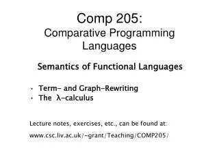
Comp 205: Comparative Programming Languages. Semantics of Functional Languages Term- and Graph-Rewriting The λ-calculus Lecture notes, exercises, etc., can be found at: www.csc.liv.ac.uk/~grant/Teaching/COMP205/. Term Rewriting. A straightforward way of implementing a

Comp 205: Comparative Programming Languages
E N D
Presentation Transcript
Comp 205:Comparative Programming Languages • Semantics of Functional Languages • Term- and Graph-Rewriting • The λ-calculus • Lecture notes, exercises, etc., can be found at: • www.csc.liv.ac.uk/~grant/Teaching/COMP205/
Term Rewriting A straightforward way of implementing a functional programming language is to implement term-rewriting. The Haskell interpreter evaluates expressions (terms) by "substituting equals for equals".
For example, given the following definitions: fib 0 = 1 fib 1 = 1 fib n = fib (n-1) + fib (n-2), if n>1 An evaluation might proceed as follows: fib 3 (fib 2) + (fib 1) (fib 1) + (fib 0) + (fib 1) 1 + (fib 0) + (fib 1) 1 + 1 + (fib 1) 1 + 1 + 1 3
+ Fn.Appl. + Fn.Appl. Fn.Appl. fib 1 fib 0 fib 1 Terms and Trees A standard way of representing terms is as trees:
Fn.Appl. fib 1 Term Rewriting Term rewriting replaces (sub)trees: (rewrites to) 1
Rewriting Trees ... giving the new tree: + + 1 Fn.Appl. Fn.Appl. fib 0 fib 1
Side-Effects In the imperative paradigm, all evaluation can change the current state (e.g., by side-effects). int funnyCount=0; int funny(int i) { return funnyCount++ * i; } funny(2) + funny(2) // might be 0+2
Functional Expressions In the functional paradigm there is no state, so an expression always denotes the same value, and evaluation simply converts an expression to its value. This important property of functional languages is referred to as "referential transparency".
Referential Transparency Referential Transparency: any expression denotes a single value, irrespective of its context. Consequently, (sub)expressions can be replaced by their values without changing the behaviour of a program. (Referential transparency = no side-effects)
Graphs Expressions can also be represented by graphs: + + Fn.Appl. Fn.Appl. fib 0 fib 1
+ + + + Fn.Appl. Fn.Appl. Fn.Appl. 1 fib 0 fib 1 fib 0 Graph Rewriting This allows identical subexpressions to be rewritten "in one go": (rewrites to)
The λ-Calculus The λ-calculus was developed by the mathematician Alonzo Church as a tool to study functions and computability. The λ-calculus provides a very simple model of computable function, and inspired the designers of the first functional programming language, LISP. The λ-calculus also provides an operational semantics for functional languages.
Computability Alan Turing developed an abstract machine (the Turing Machine) and showed that it provided a universal model of computation. He showed that the Turing-computable functions were exactly the general recursive functions. Church showed that the Turing-computable functions were exactly those that could be represented in the λ-calculus (the λ-computable functions).
Church-Turing Hypothesis Both Turing and Church conjectured that their model of computability formalised the intuitive notion of mathematical computability. The Church-Turing Hypothesis states that the equivalent notions of Turing- and λ-computability capture precisely "every function that would naturally be regarded as computable".
λ-Terms • Church designed the λ-calculus as a tool to • study the fundamental notion of computable • function. He therefore sought to strip away all • but the bare essentials. • The syntax for λ-terms is accordingly very simple. • λ-terms are built from: • variables • function application • λ-abstraction (declaring formal parameters) • (and brackets)
Syntax of λ-Terms • The set Λ of λ-terms is defined by: • Λ ::= Var | Λ Λ | λVar. Λ | (Λ) • where Var is a set of variables. • Looking at each clause in turn: • variablesTypically, we use a, b, c, ..., x, y, z for variables;if we run out of variable names, we can usex', x'', x''', etc.
Syntax of λ-Terms • function applicationIf M and N are λ-terms, so too is M N ,which represents the application of M to N.(All λ-terms can be considered functions.) • λ-abstractionIf M is a λ-term, so too is λx.M,which can be thought of as a functionwith formal parameter x,and with body M.
Some Examples • x • x y • λy.(x y) • λx.λy.x y • bracketsλ-abstraction binds less tightly than functionapplication, so the last example above shouldbe read as λx.(λy.(x y)) not (λx.(λy.x)) y .Also, x y z should be read as (x y) z .
Evaluation of λ-Terms A λ-term λx.M represents a function whose formal parameter is x and whose body is M. When this function is applied to another λ-term N, as in the λ-term (λx.M) N , evaluation proceeds by replacing x with N in the body M. For example, (λx.λy.x) (λz.z) λy.λz.z In order to make this precise, we need the notions of free and boundvariables.
Free and Bound Variables Given a λ-term λx.M, we say that λ binds ocurrences of x in M. We also say that x is bound in (λx.M). A free variable is one that is not bound by a λ-abstraction. A λ-term is closed if it has no free variables.
Free Variables • Given a λ-term M, we write FV(M) for the set of • free variables in M. This set is defined as follows: • FV( x ) = { x }In a λ-term consisting of just a variable,that variable is free. • FV( M N ) = FV(M) FV(N)Function application doesn't bind variables. • FV( λx.M ) = FV(M) - { x }If x is a bound variable, then x is not free.
Evaluation of λ-Terms Given a function application of the form (λx.M) N , evaluation proceeds by replacing all free occurrences of x in the body M with N. For example, (λx.λy.x) λz.z λy.λz.z Here, the argument λz.z replaces the variable x, which is free in the body λy.x of the function being applied.
Evaluation of λ-Terms However, (λx.(λx.x)) λz.z λx.x Here, there is no substitution, since x is not free in the body λx.x.
β-Conversion In general, we write (λx.M) NβM[x N], where M[x N] denotes the result of replacing all free occurrences of x in M with N. This form of evaluation is referred to as β-conversion, for which we use the symbol β.
Example ((λx. λy. y x) (λz.z))(λu. λv. u) β ( (λy. y x)[x (λz.z)] ) (λu. λv. u) = (λy. y (λz.z))(λu. λv. u) β ( (y (λz.z))[x (λu. λv. u)] ) = (λu. λv. u) (λz.z) β λv. λz. z
α-Conversion Just as with functions, formal parameters simply serve as place-holders, representing possible arguments. In the λ-calculus, formal parameters (i.e., bound variables) can be renamed. This is referred to as α-Conversion (written α). For example, λx. λy. y α λx. λv. v α λu. λv. v
β-Conversion Again In general, we write (λx.M) NβM[x N], where M[x N] denotes the result of replacing all free occurrences of x in M with N, provided that no free variables in N become bound as a result of this substitution. For example, (λx. λy. y x) (λz.y)β λy. y (λz.y) is not allowed.
α- and β-Conversion Sometimes it is necessary to apply α-conversion before β-conversion can be applied. For example, (λx. λy. y x) (λz.y) α (λx. λu. u x) (λz.y) β (λu. u x)[x (λz.y)] = λu. u (λz.y)
η-Conversion A final reduction relation on λ-terms is η-conversion. This applies to λ-terms of the form λx. M x, where x is not free in M. Such a function takes an argument and applies M to that argument; it is therefore equal to M itself. This is the idea behind η-conversion (η): λx. M x η M provided that x is not free in M.
Example • λy. (λx. y x) η λy. y • But η-conversion is not applicable to • λx. (λy. y x) • λy. (λx. (x y) x)
Computing with λ-Terms How does the λ-calculus relate to real programming languages such as Haskell?
Summary • Key points: • λ-terms • β-conversion • α-conversion • η-conversion • Next: Computing with λ-terms