Instrumental Variables Regression
1.13k likes | 1.55k Vues
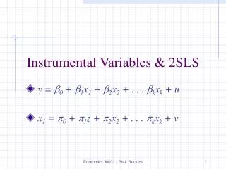
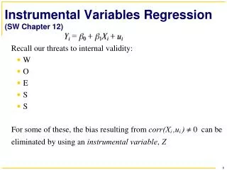
Instrumental Variables Regression. One Regressor and One Instrument The General IV Regression Model Checking Instrument Validity Application Where Do Valid Instruments Come From?. Three important threats to internal validity are:

Instrumental Variables Regression
E N D
Presentation Transcript
One Regressor and One Instrument • The General IV Regression Model • Checking Instrument Validity • Application • Where Do Valid Instruments Come From?
Three important threats to internal validity are: • omitted variable bias from a variable that is correlated with X but is unobserved, so cannot be included in the regression; • simultaneous causality bias (X causes Y , Y causes X); • errors-in-variables bias (X is measured with error). Instrumental variables regression can eliminate bias when E(u|X) ≠ 0- using an instrumental variable, Z.
One Regressor and One Instrument • Loosely, IV regression breaks X into two parts: a part that might be correlated with u, and a part that is not. By isolating the part that is not correlated with u, it is possible to estimate . • This is done using an instrumental variable, Zi , which is uncorrelated with ui . • The instrumental variable detects movements in Xi that are uncorrelated with ui , and use these to estimate .
Terminology: endogeneity and exogeneity An endogenous variable is one that is correlated with u. An exogenous variable is one that is uncorrelated with u. Historical note: • “Endogenous” literally means “determined within the system,” that is, a variable that is jointly determined with Y , or, a variable subject to simultaneous causality. • However, this definition is narrow and IV regression can be used to address OV bias and errors-in-variable bias, not just to simultaneous causality bias.
Two conditions for a valid instrument For an instrumental variable (an “instrument”) Z to be valid, it must satisfy two conditions: • Instrument relevance: Cov(Zi , Xi )≠0 • Instrument exogeneity: Cov(Zi , ui )= 0 Suppose for now that you have such a Zi (we’ll discuss how to find instrumental variables later), How can you use Zi to estimate ?
The IV Estimator, one X and one Z Explanation #1: Two Stage Least Squares (TSLS) As it sounds, TSLS has two stages - two regressions: (1)First isolates the part of X that is uncorrelated with u: regress X on Z using OLS. • Because Zi is uncorrelated with ui , is uncorrelated with ui . We don’t know or but we have estimated them. • Compute the predicted values of Xi , , where , i = 1, ... , n.
(2) Replace Xi by in the regression of interest: regress Y on using OLS: • Because is uncorrelated with ui in large samples, so the first least squares assumption holds. • Thus can be estimated by OLS using regression (2). • This argument relies on large samples (so and are well estimated using regression (1)). • This resulting estimator is called the Two Stage Least Squares (TSLS) estimator, .
Suppose you have a valid instrument, Zi . • Stage 1: Regress Xi on Zi , obtain the predicted values . • Stage 2: Regress Yi on , the coefficient on is the TSLS estimator, . Then is a consistent estimator of .
Explanation #2: Thus, where (instrument exogeneity). Thus
The IV estimator replaces these population covariances with sample covariances. sYZ and sXZ are the sample covariances This is the TSLS estimator - just a different derivation.
Consistency of the TSLS estimator The sample covariances are consistent: Thus, • The instrument relevance condition, , ensures that you don’t divide by zero.
Example #1: Supply and demand for butter IV regression was originally developed to estimate demand elasticities for agricultural goods, for example butter: • = price elasticity of butter = percent change in quantity for a 1% change in price. • Data: observations on price and quantity of butter for different years. • The OLS regression of on suffers from simultaneous causality bias (why?)
Simultaneous causality bias in the OLS regression of on arises because price and quantity are determined by the interaction of demand and supply.
This interaction of demand and supply produces Would a regression using these data produce the demand curve? No!
What would you get if only supply shifted? TSLS estimates the demand curve by isolating shifts in price and quantity that arise from shifts in supply. Z is a variable that shifts supply but not demand.
TSLS in the supply-demand example: Let Z = rainfall in dairy-producing regions. Is Z a valid instrument? • Exogenous? ? Plausibly: whether it rains in dairy-producing regions shouldn’t affect demand. • Relevant? ? Plausibly: insufficient rainfall means less grazing means less butter.
Zi = raini = rainfall in dairy-producing regions. • Stage 1: regress on raini , get . isolates changes in log price that arise from supply (part of supply, at least). • Stage 2: regress on . The regression counterpart of using shifts in the supply curve to trace out the demand curve.
Example #2: Test scores and class size • The California regressions still could have OV bias (e.g. parental involvement). • This bias could be eliminated by using IV regression (TSLS). • IV regression requires a valid instrument, that is, an instrument that is: • relevant: . • exogenous: .
Here is a (hypothetical) instrument: • some districts, randomly hit by an earthquake, “double up” classrooms: Zi = Quakei = 1 if hit by quake, = 0 otherwise. • Do the two conditions for a valid instrument hold? • The earthquake makes it as if the districts were in a random assignment experiment. Thus the variation in STR arising from the earthquake is exogenous. • The first stage of TSLS regresses STR against Quake, thereby isolating the part of STR that is exogenous (the part that is “as if” randomly assigned).
Inference using TSLS • In large samples, the sampling distribution of the TSLS estimator is normal. • Inference (hypothesis tests, confidence intervals) proceeds in the usual way, e.g. ±1.96SE. • The idea behind the large-sample normal distribution of the TSLS estimator is that - like all the other estimators we have considered - it involves an average of mean zero i.i.d. random variables, to which we can apply the CLT. • See SW App. 12.3 for the details.
Substitute in and simplify,
Thus Subtract from each side and we get,
Multiplying through by and making the approximation that yields:
First consider the numerator, in large samples, • Next consider the denominator: where because the instrument is relevant by assumption.
Statistical inference proceeds in the usual way. • The justification is (as usual) based on large samples. • This all assumes that the instruments are valid - we’ll discuss what happens if they aren’t valid later. • Important note on standard errors: • The OLS standard errors from the second stage regression are not correct— they don’t take into account the estimation in the first stage ( is estimated). • Instead, use a single specialized command that computes the TSLS estimator and the correct SEs. • As usual, use heteroskedasticity-robust SEs.
A complete digression: The early history of IV regression • How much money would be raised by an import tariff on animal and vegetable oils (butter, flaxseed oil, soy oil, etc.)? • To do this calculation you need to know the elasticities of supply and demand, both domestic and foreign. • This problem was first solved in Appendix B ofWright (1928), “The Tariff on Animal and Vegetable Oils.”
Who wrote Appendix B of PhilipWright (1928)? …this appendix is thought to have been written with or by his son, SewallWright, an important statistician. (SW, p.425) Who were these guys and what’s their story?
Example: Demand for Cigarettes • How much will a hypothetical cigarette tax reduce cigarette consumption? • To answer this, we need the elasticity of demand for cigarettes, that is, 1 in the regression, • Will the OLS estimator plausibly be unbiased? Why or why not?
Panel data: • Annual cigarette consumption and average prices paid (including tax). • 48 continental US states, 1985-1995. Proposed instrumental variable: • Zi = general sales tax per pack in the state = SalesTaxi . • Is this a valid instrument? • Relevant? ? • Exogenous? ?
For now, use data for 1995 only. First stage OLS regression: = 4.63+.031SalesTaxi , n=48 Second stage OLS regression with correct, heteroskedasticity-robust standard errors.
Summary of IV Regression with a Single X and Z • A valid instrument Z must satisfy two conditions: • relevance: • exogeneity: • TSLS proceeds by first regressing X on Z to get , then regressing Y on . • The key idea is that the first stage isolates part of the variation in X that is uncorrelated with u. • If the instrument is valid, then the large-sample sampling distribution of the TSLS estimator is normal, so inference proceeds as usual.
The General IV Regression Model • So far we have considered IV regression with a single endogenous regressor (X) and a single instrument (Z). • We need to extend this to: • multiple endogenous regressors (X1 , … , Xk). • multiple included exogenous variables (W1 , … , Wr ). These need to be included for the usual OV reason. • multiple instrumental variables (Z1 , … , Zm). More (relevant) instruments can produce a smaller variance of TSLS: the R2 of the first stage increases, so you have more variation in .
Example: cigarette demand • Another determinant of cigarette demand is income; omitting income could result in omitted variable bias. • Cigarette demand with one X, one W, and 2 instruments (2 Z’s): Z1i = general sales tax component only Z2i = cigarette-specific tax component only • Other W’s might be state effects and/or year effects (in panel data).
The general IV regression model: • Yi is the dependent variable. • X1i , … , Xki are the endogenous regressors (potentially correlated with ui ). • W1i , … , Wri are the included exogenous variables or included exogenous regressors (uncorrelated with ui ). • are the unknown regression coefficients. • Z1i , … , Zmi are the m instrumental variables (the excluded exogenous variables).
Identification • In general, a parameter is said to be identified if different values of the parameter would produce different distributions of the data. • In IV regression, whether the coefficients are identified depends on the relation between the number of instruments (m) and the number of endogenous regressors (k). • Intuitively, if there are fewer instruments than endogenous regressors, we can’t estimate . • For example, suppose k = 1 but m = 0 (no instruments)!
The coefficients are said to be: • exactly identified if m = k. There are just enough instruments to estimate • overidentified if m > k. There are more than enough instruments to estimate 1 . If so, you can test whether the instruments are valid (a test of the “overidentifying restrictions”) - we’ll return to this later. • underidentified if m < k. There are too few enough instruments to If so, you need to get more instruments!
General IV regression: TSLS, 1 endogenous regressor • Instruments: Z1i , … , Zmi . • First stage • Regress X1 on all the exogenous regressors: regress X1 on W1 , … ,Wr ; Z1 , … ,Zm by OLS. • Compute predicted values , i = 1 , … ,n. • Second stage • Regress Y on , W1 , … ,Wr by OLS. • The coefficients from this second stage regression are the TSLS estimators, but SEs are wrong. • To get correct SEs, do this in a single step.
Example: Demand for cigarettes Z1i = general sales taxi Z2i = cigarette specific taxi • Endogenous variable: (“one X”). • Included exogenous variable: ln(Incomei ) (“one W”). • Instruments (excluded endogenous variables): general sales tax, cigarette specific tax (“two Zs”). • Is the demand elasticity 1 overidentified, exactly identified, or underidentified?