Neural Networks
270 likes | 667 Vues
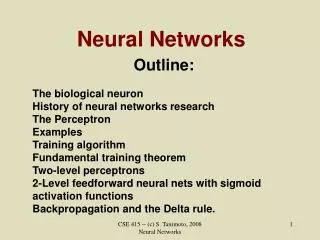
Neural Networks. Outline: The biological neuron History of neural networks research The Perceptron Examples Training algorithm Fundamental training theorem Two-level perceptrons 2-Level feedforward neural nets with sigmoid activation functions Backpropagation and the Delta rule.

Neural Networks
E N D
Presentation Transcript
Neural Networks Outline: The biological neuron History of neural networks research The Perceptron Examples Training algorithm Fundamental training theorem Two-level perceptrons 2-Level feedforward neural nets with sigmoid activation functions Backpropagation and the Delta rule. CSE 415 -- (c) S. Tanimoto, 2008 Neural Networks
The Biological Neuron The human brain contains approximately 1011 neurons. Activation process: Inputs are transmitted electrochemically across the input synapses Input potentials are summed. If the potential reaches a threshold, a pulse or action potential moves down the axon. (The neuron has “fired”.) The pulse is distributed at the axonal arborization to the input synapses of other neurons. After firing, there is a refractory period of inactivity. CSE 415 -- (c) S. Tanimoto, 2008 Neural Networks
History of Neural Networks Research 1943 McCulloch & Pitts model of neuron. ni(t+1) = (j wij nj(t) - i), (x) = 1 if x 0; 0, otherwise. 1962 Frank Rosenblatt’s book gives a training algorithm for finding the weights wij from examples. 1969 Marvin Minsky and Seymour Papert publish Perceptrons, and prove that 1-layer perceptrons are incapable of computing image connectedness. 1974-89, 1982: Associated content-addressable memory. Backpropagation: Werbos 1974, Parker 1985, Rumelhart, Hinton, & Williams 1986. CSE 415 -- (c) S. Tanimoto, 2008 Neural Networks
The Perceptron w1 x1 w2 x2 y . . . wn xn thresholding output weights inputs summation y = 1 if wi xi; 0, otherwise. CSE 415 -- (c) S. Tanimoto, 2008 Neural Networks
Perceptron Examples:Boolean AND and OR. x1 1 x2 y = x1 x2 ... xk 1 . . . xk = k - 1/2 1 x1 1 x2 y = x1 x2 ... xk 1 . . . xk = 1/2 1 xi {0, 1} CSE 415 -- (c) S. Tanimoto, 2008 Neural Networks
Perceptron Examples:Boolean NOT x y = x -1 = - 1/2 xi {0, 1} CSE 415 -- (c) S. Tanimoto, 2008 Neural Networks
Perceptron Example:Template Matching xi {-1, 1} -1 -1 1 -1 -1 -1 1 -1 1 -1 = 25 - 1 1 1 1 1 1 -1 -1 -1 1 Recognizes the letter A provided the exact pattern is present. 1 -1 -1 -1 1 weights w1 through w25 CSE 415 -- (c) S. Tanimoto, 2008 Neural Networks
Perceptron Training Sets • Let X = X+ U X- be the set of training examples. • SX = X1, X2, ..., Xk, ... is a training sequence on X, provided: • (1) Each Xk is a member of X, and • (2) Each element of X occurs infinitely often in SX. • An element e occurs infinitely often in a sequence • z = z1, z2, ... • provided that for any nonzero integer i, there exists a nonnegative integer j such that there is an occurrence of e in zi, zi+1, ..., zj. CSE 415 -- (c) S. Tanimoto, 2008 Neural Networks
Perceptron Training Algorithm Let X = X+ U X- be the set of training examples. and let SX = X1, X2, ..., Xk, ... be a training sequence on X. Let wk be the weight vector at step k. Choose w0 arbitrarily. For example. w0 = (0, 0, ..., 0). At each step k, k = 0, 1, 2, . . . Classify Xk using wk. If Xk is correctly classified, take wk+1 = wk. If Xk is in X- but misclassified, take wk+1 = wk - ck Xk. If Xk is in X+ but misclassified, take wk+1 = wk + ck Xk. The sequence ck should be chosen according to the data. Overly large constant values can lead to oscillation during training. Values that are too small will increase training time. However, ck = c0/k will work for any positive c0. CSE 415 -- (c) S. Tanimoto, 2008 Neural Networks
Perceptron Limitations Perceptron training always converges if the training data X+ and X- are linearly separable sets. The boolean function XOR (exclusive or) is not linearly separable. (Its positive and negative instances cannot be separated by a line or hyperplane.) It cannot be computed by a single-layer perceptron. It cannot be learned by a single-layer perceptron. X+ = { (0, 1), (1, 0) } X- = { (0, 0), (1, 1) } X = X+ U X- x2 x1 CSE 415 -- (c) S. Tanimoto, 2008 Neural Networks
Two-Layer Perceptrons +1 x1 +1 -1 y = XOR(x1, x2) = 0.5 -1 +1 +1 = 0.5 x2 = 0.5 CSE 415 -- (c) S. Tanimoto, 2008 Neural Networks
Two-Layer Perceptrons (cont.) Two-Layer perceptrons are computationally powerful. However: they are not trainable with a method such as the perceptron training algorithm, because the threshold units in the middle level “block” updating information; there is no way to know what the correct updates to first-level weights should be. CSE 415 -- (c) S. Tanimoto, 2008 Neural Networks
How can we generalize perceptrons to get more powerful but trainable networks? Replace sharp threshold functions by smoother activation functions. CSE 415 -- (c) S. Tanimoto, 2008 Neural Networks
Two-Layer Feedforward Networks with Sigmoid Activation Functions We get: the power of 2-level perceptrons, plus the trainability of 1-level perceptrons (well, sort of). These are sometimes called (a) “backpropagation networks,” (because the training method is called backpropagation) and (b) “two-layer feedforward neural networks.” CSE 415 -- (c) S. Tanimoto, 2008 Neural Networks
Structure of a Backprop. Network CSE 415 -- (c) S. Tanimoto, 2008 Neural Networks
Hidden Node Input Activation As with perceptrons, a weighted sum is computed of values from the previous level: hj = i wij xi However the hidden node does not apply a threshold, but a sigmoid function ... CSE 415 -- (c) S. Tanimoto, 2008 Neural Networks
Sigmoid Activation Functions Instead of using threshold functions, which are neither continuous nor differentiable, we use a sigmoid function, which is a sort of smoothed threshold function. g1(h) = 1/(1 + e-h) CSE 415 -- (c) S. Tanimoto, 2008 Neural Networks
An Alternative Sigmoid Func. g2(h) = tanh(h) = (eh – e-h)/(eh + e-h) CSE 415 -- (c) S. Tanimoto, 2008 Neural Networks
Sigmoid Function Properties Both g1 and g2 are continuous and differentiable. g1(h) = 1/(1 + e-h) g1’(h) = g1(h) (1 – g1(h)) g2(h) = tanh(h) = (eh – e-h)/(eh + e-h) g2’(h) = 1 – g2(h)2 CSE 415 -- (c) S. Tanimoto, 2008 Neural Networks
Training Algorithm Each training example has the form Xi, Ti, were Xi is the vector of inputs, and Ti is the desired corresponding output vector. An epoch is one pass through the training set, with an adjustment to the networks weights for each training example. (Use the “delta rule” for each example.) Perform as many epochs of training as needed to reduce the classification error to the required level. If there are not enough hidden nodes, then training might not converge. CSE 415 -- (c) S. Tanimoto, 2008 Neural Networks
Delta Rule For each training example Xi, Ti, Compute F(Xi), the outputs based on the current weights. To update a weight wij, add wij to it, where wij = j Fj ( is the training rate.) If wij leads to an output node, then use j=(tj – Fj) g’j(hj) If wij leads to a hidden node, then use “backpropagation”: j = g’j(hj) k k wkj The k in this last formula comes from the output level, as computed above. CSE 415 -- (c) S. Tanimoto, 2008 Neural Networks
Performance of Backpropagation Backpropagation is slow compared with 1-layer perceptron training. The training rate can be set large near the beginning and made smaller in later epochs. In principle, backpropagation can be applied to networks with more than on layer of hidden nodes, but this slows the algorithm much more. CSE 415 -- (c) S. Tanimoto, 2008 Neural Networks
Setting the Number of Hidden Nodes The number of nodes in the hidden layer affects generality and convergence. If too few hidden nodes: convergence may fail. Few but not too few nodes: possibly slow convergence but good generalization Too many hidden nodes: Rapid convergence, but “overfitting” happens. Overfitting: the learned network handles the training set, but fails to generalize effectively to similar examples not in the training set. CSE 415 -- (c) S. Tanimoto, 2008 Neural Networks
Applications of 2-Layer Feedforward Neural Networks These networks are very popular as trainable classifiers for a wide variety of pattern data. Examples: Speech recognition and synthesis Visual texture classification Optical character recognition Control systems for robot actuators CSE 415 -- (c) S. Tanimoto, 2008 Neural Networks
Problems with Neural Networks • Lack of transparency -- where is the knowledge? • This is a general problem with “connectionist” AI. • Difficulty in predicting convergence • Practical applications usually are based on empirical development rather than theory. • Difficulty in scaling up. • NNs are often useful in subsystems, but highly complex systems must be carefully structured into separately trainable subsystems. CSE 415 -- (c) S. Tanimoto, 2008 Neural Networks
