Neural Networks
Neural Networks . EA C461 - Artificial Intelligence. Topics. Connectionist Approach to Learning Perceptron, Perceptron Learning. Neural Net example: ALVINN. Autonomous vehicle controlled by Artificial Neural Network Drives up to 70mph on public highways.


Neural Networks
E N D
Presentation Transcript
Neural Networks EA C461 - Artificial Intelligence
Topics • Connectionist Approach to Learning • Perceptron, Perceptron Learning
Neural Net example: ALVINN • Autonomous vehicle controlled by Artificial Neural Network • Drives up to 70mph on public highways Note: most images are from the online slides for Tom Mitchell’s book “Machine Learning”
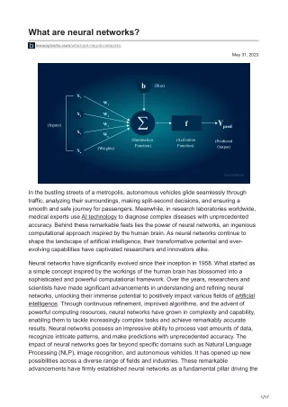
Neural Net example: ALVINN Sharp left Sharp right Straight ahead 30 output units 4 hidden units Learning means adjusting weight values 1 input pixel Input is 30x32 pixels = 960 values
Neural Net example: ALVINN • Output is array of 30 values • This corresponds to steering instructions • E.g. hard left, hard right • This shows one hidden node • Input is 30x32 array of pixel values • = 960 values • Note: no special visual processing • Size/colour corresponds to weight on link
Neural Networks • Mathematical representations of information processing in biological systems? • Efficient models for statistical pattern recognition • Multi Layer Perceptron • Model comprises multiple layers of logistic regression models (with continuous nonlinearities) • Compact models, comparing to SVM with similar generalization performances • Likelihood function is no longer convex!!! • Substantial resources requirement for training , often • Quicker processing of new data
Feed-forward Network Functions • Linear models for regression and classification • Neural networks use basis functions that follow similar form • Each basis function is itself a nonlinear function of a linear combination of the inputs, • The coefficients in the linear combination are adaptive parameters • Can be modeled as a series of functional transformations
Feed-forward Network Functions • First construct M linear combinations of the input variables x1 , . . . , xD in the form • aj is called as activation, wj0 is bias, wji are weights • h(.) – non linear differentiable transformation • Generally sigmoid function : logic sigmoid, tanh
Feed-forward Network Functions • Proceed to do the same with the second layer • The choice of activation function at second layer (corresponds to output ) is determined by the nature of the data and the assumed distribution of target variables
Feed-forward Network Functions • Evaluating this equation can be interpreted as a forward propagation of information through the network • Bias can be absorbed into the input
Activation functions • Activation functions are linear for perceptrons • Activation functions are not linear for MLP • Composition of successive linear transformations is itself a linear transformation • We can always find an equivalent network without hidden units • If the number of hidden units is smaller than either the number of input or output units, then • the information is lost in the dimensionality reduction at the hidden units. • the transformations that the network can generate are not the most general possible linear transformations from inputs to outputs because • Little / no interest in MLP’s with linear activation for hidden layers
Output layer • For regression we use linear outputs and a sum-of-squares error, for (multiple independent) • For binary classifications we use logistic sigmoid outputs and a cross-entropy error function, and for multiclass classification we use softmax outputs with the corresponding multiclass cross-entropy error function • For classification problems involving two classes, we can use a single logistic sigmoid output, or a network with two outputs having a softmax output activation function
Universal Approximators • A two-layer network with linear outputs can uniformly approximate any continuous function on a compact input domain to arbitrary accuracy provided the network has a sufficiently large number of hidden units • Universal approximators
Parameter optimization • In the neural networks literature, it is usual to consider the minimization of an error function rather than the maximization of the (log) likelihood • Maximizing the likelihood function is equivalent to minimizing the sum-of-squares error function
Parameter optimization • The value of w found by minimizing E( w ) will be denoted wML because it corresponds to the maximum likelihood solution. • The nonlinearity of the network function y( xn, w ) causes the error E( w ) to be nonconvex • In practice local maxima of the likelihood may be found,
Parameter optimization • If we make a small step in weight space from w to w+δ w then the change in the error function is δE≈ δwT∇E(w) where ∇E(w) points in the direction of greatest rate of increase of the error function. • A step in the direction of −∇E(w) reduces the error
Parameter optimization • E(w) is a smooth continuous function of w • It’s value will be smaller where the gradient of the error function vanishes , i.e E(w) = 0 , stationary point • Stationary points can be minima, maxima & saddle points • Many points in weight space at which the gradient vanishes • For any point w that is a local minimum, there will be other points in weight space that are equivalent minima • In a two-layer network with M hidden units, each point in weight space is a member of a family of M!2M equivalent points (plus) multiple inequivalent stationary points and multiple inequivalent minima
Parameter optimization • Not always feasible to find the global minimum • Also, it will not be known whether the global minimum has been found • It may be necessary to compare several local minima in order to find a sufficiently good solution • Iterative numerical procedures • Choose some initial value w(0) for the weight vector • Navigate through weight space in a succession of steps of the form w (τ +1)= w(τ)+ ∆w(τ) τ – Iteration Step • The value of ∇E(w) is evaluated at the new weight vector w(τ+1)
Gradient descent optimization • Update weight to make a small step in the direction of the negative gradient • Error function is defined with respect to a training set • Each step requires that the entire training set be processed to evaluate ∇E • Batch methods • It is necessary to run gradient-based algorithm multiple times • Each time using a different randomly chosen starting point • Comparing the resulting performance on an independent validation set
Gradient descent optimization • Error functions based on ML principle for a set of independent observations comprise a sum of terms, one for each data point • On-line gradient descent / sequential gradient descent / stochastic gradient descent, makes an update to the weight vector based on one data point at a time • Cycle through each point/ pick random points with replacement
Regularization in Neural Networks • The generalization error is not a simple function of M due to the presence of local minima in the error function • Not always feasible to choose M by plotting
Regularization in Neural Networks • The number of input and outputs units in a neural network is determined by the dimensionality of the data set • The number M of hidden units is a free parameter that can be adjusted to give the best predictive performance
Regularization in Neural Networks • Choose a relatively large value for M and then control the complexity by the addition of a regularization term to the error function • The simplest regularizer is the quadratic • Weight decay regularizer • The effective model complexity is determined by the choice of the regularization coefficient λ
Early Stopping • Training can therefore be stopped at the point of smallest error with respect to the validation data set
Invariance • In the classification of objects in two-dimensional images, such as handwritten digits, a particular object should be assigned the same classification irrespective of its • position within the image (translation invariance) • its size (scale invariance) • If sufficiently large numbers of training patterns are available, then neural network can learn the invariance(at least approximately)
Invariance • Can we augment the training set using replicas of the training patterns, transformed according to the desired invariances
Invariance • We can simply ignore the invariance in the neural network • Invariance is built into the pre-processing by extracting features that are invariant under the required transformations • Any subsequent regression or classification system that uses such features as inputs will necessarily also respect these invariances • Build the invariance properties into the structure of a neural network Convolutional neural networks • Idea: • Extracting local features that depend only on small subregions • Merge these info in later stages of processing in order to detect higher-order features ultimately as the image as a whole
Convolutional neural networks • Build the invariance properties into the structure of a neural network Convolutional neural networks • Idea: • Extracting local features that depend only on small subregions • Merge these info in later stages of processing in order to detect higher-order features ultimately as the image as a whole
Radial Basis Function • An approach to function approximation • Learned hypothesis takes the form • k user provided constant (Number of Kernels) • xu is an intance from X. • Ku will decrease with d increases, and generally it is a Gaussian Kernel, centered at xu
Radial Basis Functions • This function can be used to describe a two-layer network • The width of each kernel σ2 can be separately specified • The network training procedure learns wi.
Radial Basis Functions • Choosing kernels • One fixed width kernel for each training point • Each kernel influences the only its neighborhood • Fits training data exactly • Choose smaller number of kernels in comparison with the number of training examples • Each kernel distributed uniformly across the space (or) guided by the EM Algorithm
Radial Basis Function • Summarization on RBF • Provides a global approximation to the target function • Represented by a linear combination of many local kernel functions • To neglect the values out of defined region(region/width) • Can be trained more efficiently