Lecture 4: Feature matching

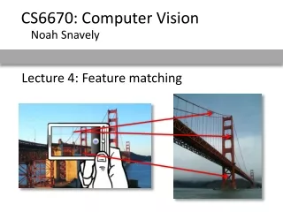
1. CS6670: Computer Vision Noah Snavely Lecture 4: Feature matching

2. The second moment matrix The surface E(u,v) is locally approximated by a quadratic form. Let’s try to understand its shape.

3. direction of the fastest change direction of the slowest change (max)-1/2 (min)-1/2 General case We can visualize H as an ellipse with axis lengths determined by the eigenvalues of H and orientation determined by the eigenvectors of H max,min: eigenvalues of H Ellipse equation:

4. Quick eigenvalue/eigenvector review The eigenvectors of a matrix A are the vectors x that satisfy: The scalar  is the eigenvalue corresponding to x • The eigenvalues are found by solving: • In our case, A = H is a 2x2 matrix, so we have • The solution: Once you know , you find x by solving

5. Corner detection: the math xmin xmax • Eigenvalues and eigenvectors of H • Define shift directions with the smallest and largest change in error • xmax = direction of largest increase in E • max = amount of increase in direction xmax • xmin = direction of smallest increase in E • min = amount of increase in direction xmin

6. Corner detection: the math • How are max, xmax, min, and xmin relevant for feature detection? • What’s our feature scoring function?

7. Corner detection: the math • How are max, xmax, min, and xmin relevant for feature detection? • What’s our feature scoring function? • Want E(u,v) to be large for small shifts in all directions • the minimum of E(u,v) should be large, over all unit vectors [u v] • this minimum is given by the smaller eigenvalue (min) of H

8. Interpreting the eigenvalues Classification of image points using eigenvalues of M: 2 “Edge” 2 >> 1 “Corner”1 and 2 are large,1 ~ 2;E increases in all directions 1 and 2 are small;E is almost constant in all directions “Edge” 1 >> 2 “Flat” region 1

9. Corner detection summary • Here’s what you do • Compute the gradient at each point in the image • Create the H matrix from the entries in the gradient • Compute the eigenvalues. • Find points with large response (min> threshold) • Choose those points where min is a local maximum as features

10. Corner detection summary • Here’s what you do • Compute the gradient at each point in the image • Create the H matrix from the entries in the gradient • Compute the eigenvalues. • Find points with large response (min> threshold) • Choose those points where min is a local maximum as features

11. The Harris operator • min is a variant of the “Harris operator” for feature detection • The trace is the sum of the diagonals, i.e., trace(H) = h11 + h22 • Very similar to min but less expensive (no square root) • Called the “Harris Corner Detector” or “Harris Operator” • Lots of other detectors, this is one of the most popular

12. The Harris operator Harris operator

13. Harris detector example

14. f value (red high, blue low)

15. Threshold (f > value)

16. Find local maxima of f

17. Harris features (in red)

18. Weighting the derivatives • In practice, using a simple window W doesn’t work too well • Instead, we’ll weight each derivative value based on its distance from the center pixel

19. Questions?

20. Harris Detector: Invariance Properties • Rotation Ellipse rotates but its shape (i.e. eigenvalues) remains the same Corner response is invariant to image rotation

21. R R x(image coordinate) x(image coordinate) Harris Detector: Invariance Properties • Affine intensity change: I aI+b • Only derivatives are used => invariance to intensity shiftI I+b • Intensity scale:I  aI threshold Partially invariant to affine intensity change

22. Harris Detector: Invariance Properties • Scaling Corner All points will be classified as edges Not invariant to scaling

23. Scale invariant detection Suppose you’re looking for corners Key idea: find scale that gives local maximum of f • in both position and scale • One definition of f: the Harris operator

24. Lindeberg et al, 1996 Lindeberg et al., 1996 Slide from Tinne Tuytelaars Slide from Tinne Tuytelaars

32. Implementation • Instead of computing f for larger and larger windows, we can implement using a fixed window size with a Gaussian pyramid (sometimes need to create in-between levels, e.g. a ¾-size image)

33. Another common definition of f • The Laplacian of Gaussian (LoG) (very similar to a Difference of Gaussians (DoG) – i.e. a Gaussian minus a slightly smaller Gaussian)

34. Laplacian of Gaussian • “Blob” detector • Find maxima and minima of LoG operator in space and scale minima * = maximum

35. Scale selection • At what scale does the Laplacian achieve a maximum response for a binary circle of radius r? r image Laplacian

36. Characteristic scale • We define the characteristic scale as the scale that produces peak of Laplacian response characteristic scale T. Lindeberg (1998). "Feature detection with automatic scale selection."International Journal of Computer Vision30 (2): pp 77--116.

37. Scale-space blob detector: Example

38. Scale-space blob detector: Example

39. Scale-space blob detector: Example

40. Questions?

41. Feature descriptors We know how to detect good points Next question: How to match them? Answer: Come up with a descriptor for each point, find similar descriptors between the two images ?

42. How to achieve invariance Need both of the following: • Make sure your detector is invariant 2. Design an invariant feature descriptor • Simplest descriptor: a single 0 • What’s this invariant to? • Next simplest descriptor: a square window of pixels • What’s this invariant to? • Let’s look at some better approaches…

43. Rotation invariance for feature descriptors • Find dominant orientation of the image patch • This is given by xmax, the eigenvector of H corresponding to max (the larger eigenvalue) • Rotate the patch according to this angle Figure by Matthew Brown

44. Multiscale Oriented PatcheS descriptor Take 40x40 square window around detected feature • Scale to 1/5 size (using prefiltering) • Rotate to horizontal • Sample 8x8 square window centered at feature • Intensity normalize the window by subtracting the mean, dividing by the standard deviation in the window 40 pixels 8 pixels CSE 576: Computer Vision Adapted from slide by Matthew Brown

45. Detections at multiple scales

46. Scale Invariant Feature Transform • Basic idea: • Take 16x16 square window around detected feature • Compute edge orientation (angle of the gradient - 90) for each pixel • Throw out weak edges (threshold gradient magnitude) • Create histogram of surviving edge orientations angle histogram 2 0 Adapted from slide by David Lowe

47. SIFT descriptor • Full version • Divide the 16x16 window into a 4x4 grid of cells (2x2 case shown below) • Compute an orientation histogram for each cell • 16 cells * 8 orientations = 128 dimensional descriptor Adapted from slide by David Lowe

48. Properties of SIFT Extraordinarily robust matching technique • Can handle changes in viewpoint • Up to about 60 degree out of plane rotation • Can handle significant changes in illumination • Sometimes even day vs. night (below) • Fast and efficient—can run in real time • Lots of code available • http://people.csail.mit.edu/albert/ladypack/wiki/index.php/Known_implementations_of_SIFT

49. SIFT Example sift 868 SIFT features

50. Feature matching Given a feature in I1, how to find the best match in I2? • Define distance function that compares two descriptors • Test all the features in I2, find the one with min distance