Download
1 / 34
340 likes | 368 Vues
Explore solutions to algebraic, differential, and integral equations involving physical parameters, with a focus on linear and nonlinear equations. Learn about bisection, false-position, fixed-point iteration, and Newton-Raphson methods.

E N D
Solution of Nonlinear Equation Dr. Asaf Varol avarol@mix.wvu.edu
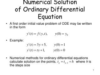
Introduction • Solutions to algebraic, differential, and integral equations relating certain physical parameters for a given problem • Algebraic equations divided into two categories: (1) Linear and (2) Nonlinear • Linear: an equation which contains the first power of the unknown, explicitly or implicitly, indicating a linear variation of the unknown parameter as a function of the other known parameters. • Example: distance, s, traveled by an object which was originally at a location s = s0 at time t = 0, and moving at constant speed, v, is related to time by s = s0 + vt • which is a linear relationship between s and v , and also between s and t since v is assumed not changing with time.
Introduction (Cont’d) • Nonlinear: an equation involving variables which contains at least one term with an exponent other than unity and/or any explicit or implicit non-linear function of that particular parameter which we want to solve for. • Example: Suppose that dv/dt = constant = a 0, i.e. there is a constant acceleration (or a body force such as gravity) acting on the object, then the relation between s and t becomes s = s0 + v0t + (a/2)t2 • where v0 is the initial speed. This equation has a nonlinear relationship between the distance, s, and the time, t, because it involves the square of the parameter t. • Example: the following relation between the angle, , of a pendulum at time, t, is a nonlinear relation. = 0cos(t) where = (g/L)1/2 is the frequency of the oscillations , 0 is the initial starting angle , g is the acceleration of the gravity, and L is the length of the connecting rod. This equation is nonlinear because the trigonometric function cos() is a nonlinear function.
Introduction (Cont’d) • Case for an object with changing acceleration as a result of drag • Case of motion of an object which was thrown vertically upward with an initial velocity of v0 = 100 m/s; hence b0 = -g = -9.8 m/s2; let c = 0.1 (1/s) and s0 = 0
Graphical Method and Scanning for t=-10:30 ft=(1-exp(-0.1*t)-0.05*t) plot(t,ft,'r*') hold on grid on end xlabel('t(sec)') ylabel('F(t)')
Graphical Method and Scanning (Cont’d) for t=-10:30 ft1=exp(-0.1*t) ft2=1-0.05*t plot(t,ft1,'r*',t,ft2,'b+') hold on end text(10,2.5,'* f(t)=exp(-0.1t)') text(10.,2.2,'+ f(t)=1-0.05t') xlabel('t(sec)') ylabel('F(t)')
Bisection Method • Bisection is a systematic search technique for finding a zero of a continuous function. The method is based on first finding an interval in which a zero is known to occur because the function has opposite signs at the ends of the interval, then dividing the interval into two equal subintervals, and determining which subinterval contains a zero, and continuing the computations on the subinterval that contains the zero. • Suppose that an interval [a, b] has been located which is known to contain a zero, since the function changes signs between a and b. The midpoint of the interval is m=(a+b)/2 and a zero must lie in either [a, m] or [m, b].
Bisection method • The appropriate subinterval is determined by testing the function to see whether it changes sign on [a, m]. If so, the search continues on that interval; otherwise, it continues on the interval [m, b]. Figure illustrates the first approximation to the zero of the function • Y=f(x)=x2-3, starting with the interval [1, 2] [2].
Example (Cont’d) • It is convenient to keep track of the calculations in tabular form.
Bisection Method (sometimes does not work at all) • Bisection method frequently converges slowly and sometimes does not work at all.
False-Position (Regula Falsi) Method • False-Position (or Regula-Falsi) Method is similar to the bisection method, with a slight improvement in the convergence rate. • Upper and lower bound of the root are used to locate a usually better estimate.
False-Position Method (Cont’d) • However, there are special cases where the false-position method does not give a better estimate than bisection method.
Fixed-Point Iteration Method • Simplest method for finding roots of nonlinear equations (also known as the “Simple Iteration Method”) • Equations need to be of the form a = g(a) • Example: F(x) = x – ln (4 + x) = 0 can be rearranged to x = ln (4 + x) = f(x) • General Iteration Procedure: xi+1 = f(xi)
Newton-Raphson Method Newton-Raphson method can be derived using a Taylor series expansion about the point x = xi F(xi+1) = F(xi) + F(xi)h + F(xi)h2/2 + F(xi)h3/6 + ... where xi+1 is the next estimate to the root, and h = xi+1 - xi • If the next iterate (xi+1) is approximately the root, then F(xi+1) 0 • The Newton-Raphson method is obtained by truncating the Taylor series at the second term and solving for xi+1
Newton-Raphson Method (Cont’d) • Error - the error is determined from the leading truncation error of the Taylor series. where Ei = xr - xi is the error in the previous iteration and Ei+1 is the error in the current iteration • Convergence - such that successive errors become smaller, the convergence of the method is sufficient that • Since the error in the next iteration is proportional to the square of the error is the previous iteration, the Newton-Raphson method has quadratic convergence, and thus is a second-order method
References • Celik, Ismail, B., “Introductory Numerical Methods for Engineering Applications”, Ararat Books & Publishing, LCC., Morgantown, 2001 • Fausett, Laurene, V. “Numerical Methods, Algorithms and Applications”, Prentice Hall, 2003 by Pearson Education, Inc., Upper Saddle River, NJ 07458 • Rao, Singiresu, S., “Applied Numerical Methods for Engineers and Scientists, 2002 Prentice Hall, Upper Saddle River, NJ 07458 • Mathews, John, H.; Fink, Kurtis, D., “Numerical Methods Using MATLAB” Fourth Edition, 2004 Prentice Hall, Upper Saddle River, NJ 07458 • Varol, A., “Sayisal Analiz (Numerical Analysis), in Turkish, Course notes, Firat University, 2001