Methods for Solving Nonlinear Equations
500 likes | 576 Vues
Learn analytical, graphical, numerical methods for root finding problems in science and engineering. Understand bracketing and open methods with convergence analysis and examples.

Methods for Solving Nonlinear Equations
E N D
Presentation Transcript
Lecture 4Solution of Nonlinear Equations( Root finding Problems ) Definitions Examples Classification of methods Analytical solutions Graphical methods Numerical methods Bracketing methods Open methods Convergence Notations Reading Assignment: Sections 5.1 and 5.2 (c)AL-DHAIFALLAH1435
Root finding Problems Many problems in Science and Engineering are expressed as These problems are called root finding problems (c)AL-DHAIFALLAH1435
Roots of Equations A number r that satisfies an equation is called a root of the equation. (c)AL-DHAIFALLAH1435
Zeros of a function Let f(x) be a real-valued function of a real variable. Any number r for which f(r)=0 is called a zero of the function. Examples: 2 and 3 are zeros of the function f(x) = (x-2)(x-3) (c)AL-DHAIFALLAH1435
Graphical Interpretation of zeros • The real zeros of a function f(x) are the values of x at which the graph of the function crosses (or touches ) the x-axis. f(x) Real zeros of f(x) (c)AL-DHAIFALLAH1435
Multiple zeros (c)AL-DHAIFALLAH1435
Multiple Zeros (c)AL-DHAIFALLAH1435
Simple Zeros (c)AL-DHAIFALLAH1435
Facts • Any nth order polynomial has exactly n zeros (counting real and complex zeros with their multiplicities). • Any polynomial with an odd order has at least one real zero. • If a function has a zero at x=r with multiplicity m then the function and its first (m-1) derivatives are zero at x=r and the mth derivative at r is not zero. (c)AL-DHAIFALLAH1435
Roots of Equations & Zeros of function (c)AL-DHAIFALLAH1435
Solution Methods Several ways to solve nonlinear equations are possible. • Analytical Solutions • possible for special equations only • Graphical Solutions • Useful for providing initial guesses for other methods • Numerical Solutions • Open methods • Bracketing methods (c)AL-DHAIFALLAH1435
Solution Methods:Analytical Solutions Analytical Solutions are available for special equations only. (c)AL-DHAIFALLAH1435
Graphical Methods • Graphical methods are useful to provide an initial guess to be used by other methods Root 2 1 1 2 (c)AL-DHAIFALLAH1435
Bracketing Methods • In bracketing methods, the method starts with an interval that contains the root and a procedure is used to obtain a smaller interval containing the root. • Examples of bracketing methods : • Bisection method • False position method (c)AL-DHAIFALLAH1435
Open Methods • In the open methods, the method starts with one or more initial guess points. In each iteration a new guess of the root is obtained. • Open methods are usually more efficient than bracketing methods • They may not converge to a root. (c)AL-DHAIFALLAH1435
Solution Methods Many methods are available to solve nonlinear equations • Bisection Method • Newton’s Method • Secant Method • False position Method • Muller’s Method • Bairstow’s Method • Fixed point iterations • ………. These will be covered in EE3561 (c)AL-DHAIFALLAH1435
Convergence Notation (c)AL-DHAIFALLAH1435
Convergence Notation (c)AL-DHAIFALLAH1435
Speed of convergence • We can compare different methods in terms of their convergence rate. • Quadratic convergence is faster than linear convergence. • A method with convergence order q converges faster than a method with convergence order p if q>p. • A Method of convergence order p>1 are said to have super linear convergence. (c)AL-DHAIFALLAH1435
Bisection Method The Bisection Algorithm Convergence Analysis of Bisection Method Examples Reading Assignment: Sections 5.1 and 5.2 (c)AL-DHAIFALLAH1435
Introduction: • The Bisection method is one of the simplest methods to find a zero of a nonlinear function. • It is also called interval halving method. • To use the Bisection method, one needs an initial interval that is known to contain a zero of the function. • The method systematically reduces the interval. It does this by dividing the interval into two equal parts, performs a simple test and based on the result of the test half of the interval is thrown away. • The procedure is repeated until the desired interval size is obtained. (c)AL-DHAIFALLAH1435
Intermediate Value Theorem • Let f(x) be defined on the interval [a,b], • Intermediate value theorem: if a function is continuous and f(a) and f(b) have different signs then the function has at least one zero in the interval [a,b] f(a) a b f(b) (c)AL-DHAIFALLAH1435
Examples • If f(a) and f(b) have the same sign, the function may have an even number of real zeros or no real zero in the interval [ a,b] • Bisection method can not be used in these cases a b The function has four real zeros a b The function has no real zeros (c)AL-DHAIFALLAH1435
Two more Examples • If f(a) and f(b) have different signs, the function has at least one real zero • Bisection method can be used to find one of the zeros. a b The function has one real zero a b The function has three real zeros (c)AL-DHAIFALLAH1435
Bisection Method • If the function is continuous on [a,b] and f(a) and f(b) have different signs, Bisection Method obtains a new interval that is half of the current interval and the sign of the function at the end points of the interval are different. • This allows us to repeat the Bisection procedure to further reduce the size of the interval. (c)AL-DHAIFALLAH1435
Bisection Algorithm Assumptions: • f(x) is continuous on [a,b] • f(a) f(b) < 0 Algorithm: Loop 1. Compute the mid point c=(a+b)/2 2. Evaluate f(c ) 3. If f(a) f(c) < 0 then new interval [a, c] If f(a) f( c) > 0 then new interval [c, b] End loop f(a) c b a f(b) (c)AL-DHAIFALLAH1435
Bisection Method Assumptions: Given an interval [a,b] f(x) is continuous on [a,b] f(a) and f(b) have opposite signs. These assumptions ensures the existence of at least one zero in the interval [a,b] and the bisection method can be used to obtain a smaller interval that contains the zero. (c)AL-DHAIFALLAH1435
Bisection Method b0 a0 a1 a2 (c)AL-DHAIFALLAH1435
Example + + - + - - + + - (c)AL-DHAIFALLAH1435
Flow chart of Bisection Method Start: Given a,b and ε u = f(a) ; v = f(b) c = (a+b) /2 ; w = f(c) no yes is (b-a) /2<ε is u w <0 no Stop yes b=c; v= w a=c; u= w (c)AL-DHAIFALLAH1435
Example Answer: (c)AL-DHAIFALLAH1435
Example: Answer: (c)AL-DHAIFALLAH1435
Best Estimate and error level Bisection method obtains an interval that is guaranteed to contain a zero of the function Questions: • What is the best estimate of the zero of f(x)? • What is the error level in the obtained estimate? (c)AL-DHAIFALLAH1435
Best Estimate and error level The best estimate of the zero of the function is the mid point of the last interval generated by the Bisection method. (c)AL-DHAIFALLAH1435
Stopping Criteria Two common stopping criteria • Stop after a fixed number of iterations • Stop when the absolute error is less than a specified value How these criteria are related? (c)AL-DHAIFALLAH1435
Stopping Criteria (c)AL-DHAIFALLAH1435
Convergence Analysis (c)AL-DHAIFALLAH1435
Convergence AnalysisAlternative form (c)AL-DHAIFALLAH1435
Example (c)AL-DHAIFALLAH1435
Example • Use Bisection method to find a root of the equation x = cos (x) with absolute error <0.02 (assume the initial interval [0.5,0.9]) Question 1: What is f (x) ? Question 2: Are the assumptions satisfied ? Question 3: How many iterations are needed ? Question 4: How to compute the new estimate ? (c)AL-DHAIFALLAH1435
Bisection MethodInitial Interval f(a)=-0.3776 f(b) =0.2784 a =0.5 c= 0.7 b= 0.9 (c)AL-DHAIFALLAH1435
ExampleSteps 1 and 2 -0.3776 -0.06480.2784 Error < 0.1 0.5 0.7 0.9 -0.06480.1033 0.2784 Error < 0.05 0.7 0.8 0.9 (c)AL-DHAIFALLAH1435
ExampleSteps 3 and 4 -0.06480.0183 0.1033 Error < 0.025 0.7 0.75 0.8 -0.0648 -0.02350.0183 Error < .0125 0.70 0.725 0.75 (c)AL-DHAIFALLAH1435
Summary of Solution • Initial interval containing the root [0.5,0.9] • After 4 iterations • Interval containing the root [0.725 ,0.75] • Best estimate of the root is 0.7375 • | Error | < 0.0125 (c)AL-DHAIFALLAH1435
Programming Bisection Method c = 0.7000 fc = -0.0648 c = 0.8000 fc = 0.1033 c = 0.7500 fc = 0.0183 c = 0.7250 fc = -0.0235 a=.5; b=.9; u=a-cos(a); v= b-cos(b); for i=1:5 c=(a+b)/2 fc=c-cos(c) if u*fc<0 b=c ; v=fc; else a=c; u=fc; end end (c)AL-DHAIFALLAH1435
Example Find the root of (c)AL-DHAIFALLAH1435
Example (c)AL-DHAIFALLAH1435
Advantages Simple and easy to implement One function evaluation per iteration The size of the interval containing the zero is reduced by 50% after each iteration The number of iterations can be determined a priori No knowledge of the derivative is needed The function does not have to be differentiable Disadvantage Slow to converge Good intermediate approximations may be discarded Bisection Method (c)AL-DHAIFALLAH1435