Download
1 / 43
430 likes | 445 Vues
This paper explores the design of "universal" scheduling algorithms that can work on general time-varying networks without knowledge of the future. It proposes a backpressure/max-weight algorithm that achieves utility close to an ideal algorithm with perfect future knowledge.

E N D
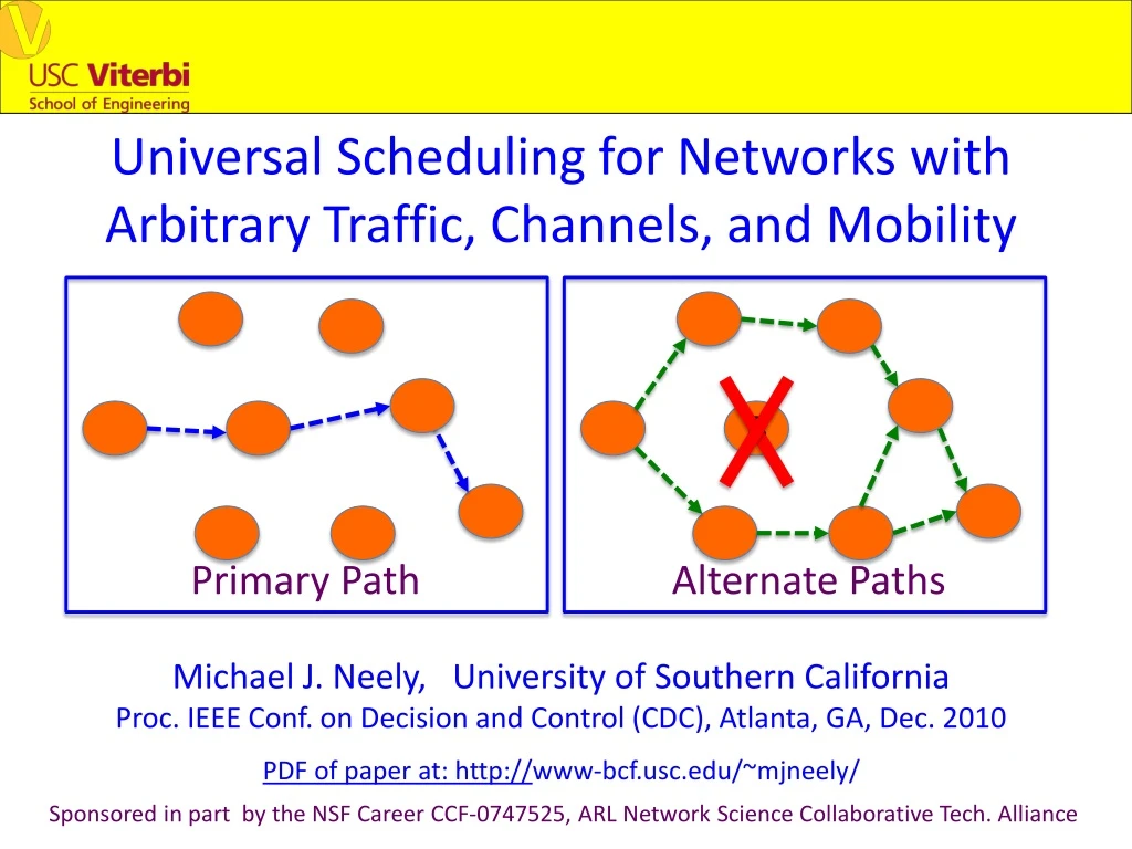
Universal Scheduling for Networks with Arbitrary Traffic, Channels, and Mobility B Primary Path Alternate Paths Michael J. Neely, University of Southern California Proc. IEEE Conf. on Decision and Control (CDC), Atlanta, GA, Dec. 2010 PDF of paper at: http://www-bcf.usc.edu/~mjneely/ Sponsored in part by the NSF Career CCF-0747525, ARL Network Science Collaborative Tech. Alliance
Want to optimally react to unexpected events. Example 1: Failure at Node B C A B D C A B D Primary Path Alternate Paths
Example 2: Opportunity via Mobility mobile node Primary Path C A B D
Example 2: Opportunity via Mobility mobile node Primary Path C A B D
Example 2: Opportunity via Mobility mobile node Primary Path C A B D
Example 2: Opportunity via Mobility mobile node Primary Path C A B D
Example 2: Opportunity via Mobility mobile node Primary Path C A B D
Example 2: Opportunity via Mobility mobile node Primary Path C A B D
Example 2: Opportunity via Mobility mobile node Primary Path C A B D
Example 2: Opportunity via Mobility mobile node Primary Path C A B D
Example 2: Opportunity via Mobility mobile node Primary Path C A B D
Example 2: Opportunity via Mobility mobile node Primary Path C A B D
Example 2: Opportunity via Mobility mobile node Primary Path C A B D
Example 2: Opportunity via Mobility mobile node Primary Path C A B D
Assumptions and Main Questions: • Assumptions: • Arbitrary mobility, traffic, channels. • Little or no probability models known in advance. • Any sample path is possible (non-ergodic). • Future is unknown. • Questions: • Can we design “universal” scheduling algorithms • that work on general time-varying networks? • Can we optimize without knowing the future?
Main Results: • We use a backpressure/max-weight algorithm • that does not know future. • Define a “T-Slot Lookahead” Utility as that obtained • by an “ideal” algorithm that has perfect knowledge • of the future up to T slots. • For any T, our algorithm can achieve utility that is • arbitrarily close to the utility of the ideal T-slot Lookahead • algorithm, with tradeoff in convergence time and • queue backlog.
Problem Formulation: • Timeslotted system, slots t = {0, 1, 2, …}. • N network nodes (possibly mobile). • M Data Flows (each with source-destination). • No pre-specified routes (we learn them).
Problem Formulation: • Timeslotted system, slots t = {0, 1, 2, …}. • N network nodes (possibly mobile). • M Data Flows (each with source-destination). • No pre-specified routes (we learn them). 4 Nodes: N = 8 5 8 1 2 3 7 6
Problem Formulation: • Timeslotted system, slots t = {0, 1, 2, …}. • N network nodes (possibly mobile). • M Data Flows (each with source-destination). • No pre-specified routes (we learn them). 4 Nodes: N = 8 Flows: M = 3 5 8 1 2 3 7 6
Problem Formulation: • Timeslotted system, slots t = {0, 1, 2, …}. • N network nodes (possibly mobile). • M Data Flows (each with source-destination). • No pre-specified routes (we learn them). 4 • Nodes: N = 8 • Flows: M = 3 • Flow 1: 13 5 1 8 1 2 3 7 6
Problem Formulation: • Timeslotted system, slots t = {0, 1, 2, …}. • N network nodes (possibly mobile). • M Data Flows (each with source-destination). • No pre-specified routes (we learn them). 4 • Nodes: N = 8 • Flows: M = 3 • Flow 1: 13 • Flow 2: 73 5 1 8 1 2 3 7 6 2
Problem Formulation: • Timeslotted system, slots t = {0, 1, 2, …}. • N network nodes (possibly mobile). • M Data Flows (each with source-destination). • No pre-specified routes (we learn them). 3 4 • Nodes: N = 8 • Flows: M = 3 • Flow 1: 13 • Flow 2: 73 • Flow 3: 56 5 1 8 1 2 3 7 6 2
Problem Formulation: • Timeslotted system, slots t = {0, 1, 2, …}. • N network nodes (possibly mobile). • M Data Flows (each with source-destination). • No pre-specified routes (we learn them). 3 4 • Nodes: N = 8 • Flows: M = 3 • Flow 1: 13 • Flow 2: 73 • Flow 3: 56 5 1 8 1 2 3 7 6 2
Network Queueing: a b a • Each node keeps queues for each separate commodity (“commodity” = “destination”). • For commodity c (say, green commodity): • Qa(c)(t+1) = Qa(c)(t) – Transmit out • + Endogenous Arrivals + Exogenous Arrivals
State Information and Control Decisions: • A(t) = (A1(t), …, AM(t)) = New Arrivals. • X(t) = (X1(t), …, XM(t)) = Flow Control Decisions. • S(t) = “Topology State” observed on slot t. • (μij(c)(t)) = Transmission Decisions (in set Γ(S(t)) Node i Am(t)
State Information and Control Decisions: • A(t) = (A1(t), …, AM(t)) = New Arrivals. • X(t) = (X1(t), …, XM(t)) = Flow Control Decisions. • S(t) = “Topology State” observed on slot t. • (μij(c)(t)) = Transmission Decisions (in set Γ(S(t)) Xm(t) Node i Am(t) Dropm(t)
State Information and Control Decisions: • A(t) = (A1(t), …, AM(t)) = New Arrivals. • X(t) = (X1(t), …, XM(t)) = Flow Control Decisions. • S(t) = “Topology State” observed on slot t. • (μij(c)(t)) = Transmission Decisions (in set Γ(S(t)) Node j Xm(t) Node i Sij(t) Am(t) Dropm(t) Node k Sik(t)
State Information and Control Decisions: • A(t) = (A1(t), …, AM(t)) = New Arrivals. • X(t) = (X1(t), …, XM(t)) = Flow Control Decisions. • S(t) = “Topology State” observed on slot t. • (μij(c)(t)) = Transmission Decisions (in set Γ(S(t)) Xm(t) Sij(t) Am(t) Dropm(t) Sik(t)
Utility Maximization with T-Slot Lookahead: • φm(x) = concave utility function for flow m • Segment timeline into T-slot frames. • φopt[r] = optimal sum utility over frame r, • assuming future is known in frame! Frame 0 Frame 2 Frame 1 • Value of φopt[r] can be written as a non-linear • program (assuming future A(t), S(t) known)…
Utility Maximization with T-Slot Lookahead: Frame r • Value of φopt[r] can be written as a non-linear • program (assuming future A(t), S(t) known): Ω(t) = set of rates possible under S(t)
Analytical Approach: • Lyapunov Function for queues: L(Q) = ∑ [Qi(c)]2 • New sample path “T-slot” Lyapunov Drift: • ΔT(t) = L(Q(t+T)) – L(Q(t)) • Every slot “greedily” minimize drift-plus-penalty: • Δ1(t) + V xPenalty(t) , Penalty(t) = -φ(γ(t)) • Results in a joint backpressure and flow control • alg similar to those defined for ergodic systems in: • [Neely, Modiano, Li -- INFOCOM 2005] • [Georgiadis, Neely, Tassiulas -- F&T 2006]
Performance Result: • Theorem: For any R>0, T>0: • (ii) Worst Case Queue Backlog = O(V). • B, C are known constants. • V = “knob” to turn to affect the tradeoff • R = Running Time (number of T-slot frames) Achieved Utility over RT slots ≥ (1/R)∑r=0φopt[r]– “Fudge Factor” R-1 BT + CV (i) “Fudge Factor” = V RT O(1/V), O(V) utility-backlog tradeoff when time horizon R infinity
Example Mobile Network: • Five Mobility Groups: • 10 nodes Group 1 (upper left) • 10 nodes Group 2 (upper right) • 10 nodes Group 3 (lower right) • 10 nodes Group 4 (lower left) • 1 node Group 5 D1 S1 S2 Group 1 nodes: Random Walk on Upper Left Region
Example Mobile Network: • Five Mobility Groups: • 10 nodes Group 1 (upper left) • 10 nodes Group 2 (upper right) • 10 nodes Group 3 (lower right) • 10 nodes Group 4 (lower left) • 1 node Group 5 D1 S1 S2 Group 2 nodes: Random Walk on Upper Right Region
Example Mobile Network: • Five Mobility Groups: • 10 nodes Group 1 (upper left) • 10 nodes Group 2 (upper right) • 10 nodes Group 3 (lower right) • 10 nodes Group 4 (lower left) • 1 node Group 5 D1 S1 S2 Group 3 nodes: Random Walk on Lower Right Region
Example Mobile Network: • Five Mobility Groups: • 10 nodes Group 1 (upper left) • 10 nodes Group 2 (upper right) • 10 nodes Group 3 (lower right) • 10 nodes Group 4 (lower left) • 1 node Group 5 D1 S1 S2 Group 4 nodes: Random Walk on Lower Left Region
Example Mobile Network: • Five Mobility Groups: • 10 nodes Group 1 (upper left) • 10 nodes Group 2 (upper right) • 10 nodes Group 3 (lower right) • 10 nodes Group 4 (lower left) • 1 node Group 5 D1 S1 S2 Group 5 node: Periodically cycles about the clockwise orbit
Example Mobile Network: Sim. 1– Change Social Contacts Backlog Bound for D1 in a sample RED node D1 S1 Backlog Bound for S1 in a sample RED node S2 • Social Contacts: • Source 1: S1D1 (constant rate = 0.07 packets/slot) • Source 2: S2 S1 (for first half of simulation) • S2 D1 (for second half of simulation) • Goal: Maximize Throughput of Source 2 subject to stability • Use V=10, so guarantee no more that 11 source 2 packets • in any queue!
Example Mobile Network: Sim. 1– Change Social Contacts Moving Average thruput:S2D1 D1 S1 Moving Average thruput:S2S1 S2 • Social Contacts: • Source 1: S1D1 (constant rate = 0.07 packets/slot) • Source 2: S2 S1 (for first half of simulation) • S2 D1 (for second half of simulation) • Goal: Maximize Throughput of Source 2 subject to stability • Use V=10, so guarantee no more that 11 source 2 packets • in any queue!
Example Mobile Network: Sim. 1– Change Social Contacts Moving Average thruput:S2D1 D1 S1 Moving Average thruput:S2S1 S2 • Overall Performance is Seamless: • Backlog no more than 11 packets in any queue for Source 1 data • Backlog no more than 15 packets in any queue for Source 2 data • Overall Thruput of Source 2 is maintained at near-optimal over the • change, even though the routes must fundamentally change!
Example Mobile Network: Sim. 2– Intermittent Jamming JAM! JAM! Time D1 S1 S2 • Social Contacts: • Source 1: S1D1 (constant rate = 0.07 packets/slot) • Source 2: S2 S1 (Goal to maximize its throughput) • Intermittent Interference during 2 intervals of the simulation • That completely cut interaction between the groups 1-4. • Can only use the cyclic mobile node at these times! • Max Thruput of Source 2 during interference ~= 0.03.
Example Mobile Network: Sim. 2– Intermittent Jamming D1 JAM! S1 JAM! Time S2 • Social Contacts: • Source 1: S1D1 (constant rate = 0.07 packets/slot) • Source 2: S2 S1 (Goal to maximize its throughput) • Intermittent Interference during 2 intervals of the simulation • That completely cut interaction between the groups 1-4. • Can only use the cyclic mobile node at these times! • Max Thruput of Source 2 during interference ~= 0.03.
Conclusion Slide: Backlog Bound for D1 in a sample RED node D1 S1 Backlog Bound for S1 in a sample RED node Moving Average Thruput of Source 2 S2 • Overall Seamless Operation • Throughput During Jamming goes down, • but is close to optimal value of 0.03. • Fudge Factor = BT/V + CV/RT • Worst Case Queue Backlog = O(V) • Framework useful for stock market trading! (Thursday @ 10:20am)