Download

1 / 37
390 likes | 736 Vues
Causal Diagrams and the Identification of Causal Effects. A presentation of Chapters 3 and 4 of: Judea Pearl Causality: Models, Reasoning and Inference Cambridge University Press, 2000. An Example. This is example is due to Cochran through Pearl [2000, p.66]

E N D
Causal Diagrams and the Identification of Causal Effects A presentation of Chapters 3 and 4 of: Judea Pearl Causality: Models, Reasoning and Inference Cambridge University Press, 2000
An Example This is example is due to Cochran through Pearl [2000, p.66] “Soil fumigants (X) are used to increase oat crop yields (Y) by controlling the eelworm population (Z).” Last year’s eelworm population (Z0) is an unknown quantity that is strongly correlated with this year’s population. Through laboratory analysis of soil samples, we can determine the eelworm populations before and after the treatments (Z1 and Z2). Furthermore , we assume that the fumigants do not affect the growth of eelworms surviving the treatment. Instead, eelworm’s growth depends on the population of birds (B), which is correlated with last year’s eelworm population and hence with the treatment itself. Z3 here represents the eelworm population at the end of the season.” We wish to assess the total effect of the fumigants on yields. But, controlled randomized experiment are unfeasible and Z0 is unknown. If we got a correct model, can we obtain consistent estimate of the target quantity – the total effect of the fumigants on yields – through observations? Causality: Models, Reasoning and Inference Chapter 3
Graphs as Models of Interventions • A causal diagram is a directed acyclic graph G that identifies the causal connections among the variables of interest. • The causal reading of a DAG is in terms of functional, rather than probabilistic relationships where pai are the parents of variable Xi in G. ui are mutually independent and represent unobserved factors, including random disturbances. • We have the same recursive decomposition as in a Bayesian network: Causality: Models, Reasoning and Inference Chapter 3
External Intervention & Causal Effect • The simplest type of external intervention is one in which a single variable, say Xi, is forced to take on some fixed value xi. We call such an intervention “atomic” and denote it by do(Xi =xi) or do(xi) for short. • Definition 3.2.1(Causal Effect): Given two disjoint sets of variables, X and Y, the causal effect of X on Y, denoted either as or as , is a function from X to the space of probability distributions on Y. For each realization x of X, gives the probability of Y = y induced by deleting from the model of (3.4) all equations corresponding to variables in X and substituting X=x in the remaining equations. Causality: Models, Reasoning and Inference Chapter 3
Correlation vs. Causation • The genotype theory (Fisher, 1958) of smoking and lung cancer: smoking and lung cancer are both effects of a genetic predisposition • Three node network • X( smoking) and Y( lung cancer) are in lockstep • X precedes Y in time (smoke before cancer) • But, X does not cause Y, because if we set X, Y does not change: Y only changes according to the value of U (the genotype) U X Y Causality: Models, Reasoning and Inference Chapter 3
Effect of Interventions • From definition 3.2.1, we have: • Theorem 3.2.2(adjustment for Direct causes) Let PAi denote the set of direct causes of variable Xi, and let Y be any set of variables disjoint of . The effect of the intervention on Y is given by Where and represent preintervention probabilities. Causality: Models, Reasoning and Inference Chapter 3
Causal Effect Identifiably • Definition 3.2.4(Causal Effect Identifiability) • The causal effect of X on Y is identifiable from a graph G if the quantity can be computed uniquely from any positive probability of the observed variables – that is , if for every pair of models M1 and M2 with the same probability distribution for the set of observed variables (v), i.e. and the same graph, i.e., • Theorem 3.2.5 • Given a causal diagram G of any Markovian model in which a subset V of variables are measured, the causal effect is identifiable whenever , that is, whenever X, Y, and all parents of variables in X are measured. The expression for is then obtained by adjusting for PAx, as in 3.14 • A special case of Theorem 3.2.5 holds when all variables are assumed to be observed. Causality: Models, Reasoning and Inference Chapter 3
U X Y Example of Nonidentifiability • The identifiablility of ensures that it is possible to infer the effect of action do(X=x) on Y from passive observations and the causal graph G, which specifies which variables participate in the determination of each variable in the domain. • To prove nonidentifiability, it is sufficient to present two sets of structural equations that induce identical distributions over observed variables but have different causal effects. • X,Y is observable, U is not. All of them are binary variables. • If P(X=0|U) = (0.5,0.5) • P(Y=0|X,U) = • But we don’t know P(U) • When P(U=0) = 0.5, P(Y|X=0) =(.45,.55) • When P(U=0) = 0.1, P(Y|X=0) =(.73,.27) • So, P(Y|do(X)) is non-identifiable Causality: Models, Reasoning and Inference Chapter 3
Example of Nonidentifiability • The identifiablility of ensures that it is possible to infer the effect of action do(X=x) on Y from passive observations and the causal graph G, which specifies which variables participate in the determination of each variable in the domain. • To prove nonidentifiability, it is sufficient to present two sets of conditional probability tables that induce identical distributions over observed variables but have different causal effects. • X,Y is observable, U is not. All of them are binary variables. • Let P(X,Y,U) be If P(X=0|U) = (0.5,0.5) • P(Y=0|X,U) = • But we don’t know P(U) • When P(U=0) = 0.5, P(Y|X=0) =(.45,.55) • When P(U=0) = 0.1, P(Y|X=0) =(.73,.27) • So, P(Y|do(X)) is non-identifiable U X Y Causality: Models, Reasoning and Inference Chapter 3
U X U Y X Y Fisher vs. the Surgeon General U X Y Only X and Y are observable Fisher’s Genotype Theory Surgeon General’s Opinion Causality: Models, Reasoning and Inference Chapter 3
Intervention as surgically modified DAGs Causality: Models, Reasoning and Inference Chapter 3
Different Causal Effects for the Same Observations Causality: Models, Reasoning and Inference Chapter 3
Interventions as Variables The effect of an atomic intervention do(Xi=xi’) is encoded by adding to G a link FiXi, where Fi is a new variable taking values in {do(xi’),idle}, xi’ ranges over the domain of Xi, and “idle” represents no intervention. Then we define: Causality: Models, Reasoning and Inference Chapter 3
Backdoor Criterion • If we can get P’(y|z,x,Fx) = P(y|x,z) and P’(z|Fx) =P(z), then we know is identifiable. • Definition 3.3.1(Back-Door) A set of variables Z satisfies that back-door criterion relative to an ordered pair of variables(Xi,Xj) in a DAG G if: (i) no node in Z is a descendant of Xi; and (ii) Z blocks every path between Xi and Xj that contains an arrow into Xi. Similarly, if X and Y are two disjoint subsets of nodes in G, then Z is said to satisfy that back-door criterion relative to (X,Y) if it satisfies that criterion relative to any pair (Xi,Xj) such that Xi X and Xj Y. Theorem 3.3.2(Back-Door Adjustment) If a set of variables Z satisfies the back-door criterion relative to (X,Y), then the causal effect of X on Y is identifiable and is given by the formula: Causality: Models, Reasoning and Inference Chapter 3
Backdoor Path Keshan Disease To determining the causal effect of Selenium on Keshan Disease, we need to find the variable set Z, called concomitants, which satisfies the back-door criteria. Z={ Region of China} is a answer. Z={Genotype} also, but this variable maybe is not observable. Causality: Models, Reasoning and Inference Chapter 3
Smoking and the genotype theory • Consider the relation between smoking(X) and lung cancer(Y). • the tobacco industry has managed to forestall antismoking legislation by arguing that observed correlation between smoking and lung cancer could be explained by some sort of carcinogenic genotype(U) that involves inborn carving for nicotine • here, Z is the amount of tar deposited in a person's lungs. • Can we get? Causality: Models, Reasoning and Inference Chapter 3
Effect of Smoking on Lung Cancer in the Presence of Tar Deposits • We compute • But • And, by the backdoor criterion, Causality: Models, Reasoning and Inference Chapter 3
Front-Door Criterion • Definition 3.3.3(Front-Door) A set of variables Z is said to satisfy the front-door criterion relative to an ordered pair of variables (X,Y) if: (i) Z intercepts all directed paths from X to Y; (ii) there is no back-door path from X to Z; and (iii) all back-door paths from Z to Y are blocked by X. • Theorem 3.3.4 (Front-Door Adjustment) if Z satisfies the front-door criterion relative to (X,Y) and if P(x,z) >0, then the causal effect of X on Y is identifiable and is given by the formula: Causality: Models, Reasoning and Inference Chapter 3
Proof of Front_Door Assume u is the parent set of x, from (i), we have The intervention do(x) removes the factor P(x|u) and induces the post intervention distribution. So From (ii) and (iii), we also have: So: Another proof will be given after the three rules. Causality: Models, Reasoning and Inference Chapter 3
Pearl’s Calculus of Interventions • Let X,Y and Z be arbitrary disjoint sets of nodes in a causal DAG G. We denote by the graph obtained by deleting from G all arrows pointing to nodes in X. Likewise, we denote by Gx the graph obtained by deleting from G all arrows emerging from nodes in X. to represent the deletion of both incoming and outgoing arrows, we use the notation ( see Figure 3.6 for an illustration). Finally, the expression stands for the probability of Y=y given that X is held constant at x and that (under this condition) Z=z is observed. Each of these inference rules follows from the basic interpretation of the “hat” operator as a replacement of the causal mechanism that connects X to its preaction parents by a new mechanism X =x introduced by the intervening force. The result is a sub model characterized by the subgraph Gx. Causality: Models, Reasoning and Inference Chapter 3
The Three Rules Theorem 3.4.1 ( Rules of Do calculus) Let G be the directed acyclic graph associated with a causal model as defined in(3.2), and let P(.) stand for the probability distribution induced by that model. For any disjoint subsets of variables X, Y, Z, and W, we have the following rules. Rule 1 (Insertion/deletion of observations): Rule 1 reaffirms d-separation as a valid test for conditional independence in the distribution resulting from the intervention do(X=x), hence the graph . This rule follows from the fact that deleting equations from the system does not introduce any dependencies among the remaining disturbance terms. Causality: Models, Reasoning and Inference Chapter 3
The Three Rules Rule 2 ( Action /observation exchange): Rule 2 provides a condition for an external intervention do(Z=z) to have the same effect on Y as the passive observation Z=z, The condition amounts to {XW} blocking all back-door paths form Z to Y( in ), since retains all (and only ) such paths. Causality: Models, Reasoning and Inference Chapter 3
The Three Rules Rule 3 (Insertion/deletion of actions): ,where Z(W) is the set of Z-nodes that are not ancestors of any W-node in Consider G’ with intervention arcs FZZ added. implies that So, any path from Z to Y that is not blocked by {X,W} in must end in an arrow pointing to Z, otherwise would not hold. In addition, if there is a path from some Z’ of Z to Y that does and in an arrow pointing to Z’, then W must not be a descendant of Z’, otherwise would not hold. Thus the only paths from Y to Z must end in an arrow pointing at Z, and must end in some member of Z(W). Thus, Causality: Models, Reasoning and Inference Chapter 3
Usage of the Three Rules Corollary 3.4.2 A causal effect Is identifiable in a model characterized by a graph G if there exists an finite sequence of transformations, each conforming to one of the inference rules in Theorem 3.4.1, that reduces q into a standard (i.e., “hat”-free) probability expression involving observed quantities. Whether Rules 1-3 are sufficient for deriving all identifiable causal effects remains an open question Causality: Models, Reasoning and Inference Chapter 3
The Smoking Example 1, Based on rule 2, we have Causality: Models, Reasoning and Inference Chapter 3
The Smoking Example • 2 Note: we can use the same process to prove back-door formula Causality: Models, Reasoning and Inference Chapter 3
The Smoking Example • 3 Based on 1,2, and above, we get: This is also a proof of front door formula Causality: Models, Reasoning and Inference Chapter 3
The Smoking Example • 4 See 1 and the third formula in 3, we have: 5 See 2 Causality: Models, Reasoning and Inference Chapter 3
Some Nonidentifiable Models Why c is not identifiable? Causality: Models, Reasoning and Inference Chapter 3
Some Identifiable Models Causality: Models, Reasoning and Inference Chapter 3
Why They are Identifiable • (a), (b) rule 2, • (c), (d) back-door • (e) front-door • (f) • (g) Causality: Models, Reasoning and Inference Chapter 3
Why g? • Z1 block all directed paths from X to Y • Z2 blocks all back-door paths between Y and Z1 in • Putting the pieces together, we obtain the claimed result Causality: Models, Reasoning and Inference Chapter 3
Several More Nonidentifiable Models Causality: Models, Reasoning and Inference Chapter 3
Completeness of the Three Rules • Completeness is conjectured by Pearl • Scheme for finding a counterexample • generate graphs (models) • filter identifiable models by using 3 rules • filter unidentifiable models by using edge subgraph algorithm with figure 3.9 patterns • rewrite P(y|do(x)) using the rules of probability • If some formula for P(y|do(x)) without U exists, a counterexample has been found • If no formula for P(y|do(x)) without U exists, we add the model to the patterns of figure 3.9 Causality: Models, Reasoning and Inference Chapter 3
Identify Theorem 4.3.1(Galles and Pearl 1995) Let X and Y denote two singleton variables in a semi_Markovian Model characterized by graph G. A sufficient condition for the identifiability of is that G satisfy one of the following four conditions. 1, there is no back-door path from X to Y in G. 2,There is no directed path from X to Y in G. 3,There exists a set of nodes B that bocks all back-door paths from X to Y so that is identifiable. ( A special case of this condition occurs when B consists entirely of nondescendents of X, in which case reduces immediately to P(b).) 4,There exist sets of nodes Z1 and Z2 such that: • Z1 blocks every directed path form X to Y; • Z2 blocks all back-door paths between Z1 and Y; • Z2 blocks all back-door paths between X and Z1; • Z2 does not activate any back-door paths from X to Y. this condition holds if (i)-(iii) are met and no member of Z2 is a descendant of X. (A special case of condition 4 occurs when Z2 = and there is no back-door path from X to Z1 or from Z1 to Y.) Theorem 4.3.2 the four conditions of Theorem 4.3.1 are necessary for identifiability in do calculus. Causality: Models, Reasoning and Inference Chapter 3
Remarks on Efficiency • Theorem 4.3.3 if is identifiable for one minimal blocking set Bi, then is identifiable for any other minimal set Bj. ( for condition 3) • Lemma 4.3.4 If the query is identifiable and if a set of nodes Z lies on a directed path form X to Y, then the query is identifiable. • Theorem 4.3.5 let Y1 and Y2 be two subsets of nodes such that either (i) no nodes Y1 are descendants of X or (ii) all nodes Y1 and Y2 are descendants of X and all nodes Y1 are nondescendants of Y2. A reducing sequence for exists if and only if there are reducing sequences for both and . • Theorem 4.3.6 If there exists a set Z1 that meets all of the requirements for Z1 in condition 4, then the set consisting of the children of X intersected with the ancestors of Y will also meet all of the requirements for Z1 in condition 4. Causality: Models, Reasoning and Inference Chapter 3
Closed-Form Expression for Control Queries • Function: ClosedForm( ). • Input:Control query of the form . • Output: either a closed-form expression for ,in terms of observed variables only, or FAIL when query is not identifiable. • 1, if then return P(y). • 2, Otherwise, if then return P(y|x). • 3, Otherwise, let B=BlockingSet(X,Y), and Pb=ClosedForm( ) ;if Pb!=FAIL, then return . • 4. Otherwise, let Z1=Children(X) (Y Ancestors(Y)), Z3=BlockingSet(X,Z1), Z4 = BlockingSet(Z1,Y), and Z2 = Z3 Z4; if Y Z1 and X Z2 then return • 5, Otherwise return FAIL Steps 3 and 4 invoke the function BlockingSet(X,Y), which selects a set of nodes Z that d-separate X form Y. Step 3 contains a recursive call to the algorithm ClosedForm( ) itself, in order to obtain an expression for causal effect . Causality: Models, Reasoning and Inference Chapter 3