Download

1 / 29
290 likes | 406 Vues
This guide covers the basics of servo motor control, focusing on enhancing the smoothness of movements. During your lab period from May 5-9, you will explore techniques to control motor position and velocity effectively. Through hands-on activities, you'll learn about polynomial fitting for smoothing curves and reducing choppy movements. You'll analyze various polynomial orders and practice using MATLAB to generate smooth curves based on time and velocity. By the end of your study, you'll understand the principles behind teaching a robot for precise, fluid motor control.

E N D
The Final Exam • During the last week of classes • In your lab period • May 5-9 • Tell your friends
Servo Motor Control Basic computer control of motor position and velocity
Reading • Chapter 11
watch the motor movement http://www.youtube.com/watch?v=7coUcEHxnYA - notice the choppy movement between taught points http://www.youtube.com/user/CompassAutomation?v=lpY2P4lDYwg - notice that the movements have been smoothed out
smooth movement starts slow, speeds up, finishes slow Position vs. time Velocity vs. time
How do you teach a robot? • manually stepping through specific points • the results is often "choppy", because of the selection of just a few points of travel
the problem You know "basically" where the robot arm should be, with a few points. Very choppy. To run smoothly in real time, you need thousands, actually a descriptive formula, p= f(t), and v= f(t)
we must smooth out the curve to this taught manually derived from a formula
how we solve it • Program 11 pts. Capture the (x,y) value of each point. x = [ 0 10 25 30 40 50 60 70 75 90 100 ] y = [ 0 7.5 20 30 45 50 45 30 20 7.5 0 ] remember that x represents time, and y represents velocity
Find a polynomial equation that generates the same y's, from those x's (that is, an equation that matches the x,y curve). y = ax2 + bx + c • Generate 100s of x,y points using the formula to smooth out the curve
polynomials • 2nd order: y = ax2 + bx + c • 3rd order: y = ax3 + bx2 + cx + d • 4th order: y = ax4 + bx3 + cx2 + dx + e number of coefficients = order+1
step 1 y = [0 7.5 20 30 45 50 45 30 20 7.5 0 ] x = [0 10 25 30 40 50 60 70 75 90 100 ] figure(1) plot( x, y) reflect on this.... it's very poor vel vs time, and results in choppy movement
coeff = polyfit(x, y, n) • find a polynomial of the nth order that fits the x vs y vectors • coeff will be a column vector of n+1 values • if n = 2, then MATLAB will return coeff(1), coeff(2), and coeff(3) so that • vel = coeff(1) * x2 + coeff(2) * x + coeff(3) • remember : x = [0 10 25 30 40 50 60 70 75 90 100 ] vel = [ desired 11 new pts ]
order = 2 coeff = polyfit(x,y,2) % x.^2 means x2 vel = (coeff(1)*x.^2) +(coeff(2)*x) + coeff(3) %coeff: -0.0182 1.8182 -5.0000 figure(2) plot(x, vel)
order = 3 coeff = polyfit(x,y,3) vel = (coeff(1)*x.^3)+(coeff(2)*x.^2)+(coeff(3)*x) + coeff(4) figure(3) plot(x, vel)
order = 4 (5 coeffs) coeff = polyfit(x,y,4) vel =(coeff(1)*x.^4)+(coeff(2)*x.^3)+(coeff(3)*x.^2) + (coeff(4)*x) +coeff(5) figure(4) plot(x, vel)
order = 5 (6 coeffs) coeff = polyfit(x,y,5) vel = (coeff(1)*x.^5)+(coeff(2)*x.^4)+(coeff(3)*x.^3)+(coeff(4)*x.^2)+(coeff(5)*x) + coeff(6) figure(5) plot(x, vel)
order = 6 (7 coeffs) coeff = polyfit(x,y,6) vel = (coeff(1)*x.^6)+(coeff(2)*x.^5)+(coeff(3)*x.^4)+(coeff(4)*x.^3)+(coeff(5)*x.^2)+ (coeff(6)*x)+coeff(7) figure(6) plot(x, vel)
now plot for 1000 values of X x = [1: .1 :100] vel = (coeff(1)*x.^6)+(coeff(2)*x.^5)+(coeff(3)*x.^4)+(coeff(4)*x.^3)+(coeff(5)*x.^2)+ (coeff(6)*x)+coeff(7) figure(7) plot(x, vel)
practice for the exam: %define an x row vector of 5 pts: x = [1:20:100] %get any y function of 5 pts y = 40*( 1-sin(x*pi/180) ) figure(10) plot( x, y)
polyfit to order = 2 coeff = polyfit(x,y,2) vel = (coeff(1)*x.^2)+(coeff(2)*x)+coeff(3) figure(11) plot(x, vel)
test that curve with 100 pts. x = [1:100] y = (coeff(1)*x.^2)+(coeff(2)*x)+coeff(3) figure(12) plot(x, y)
try 6th order %define an x row vector of 5 pts: x = [1:20:100] %get a y function of 5 pts y = 40*(1-sin(x*pi/180)) coeff = polyfit(x,y,6) vel = (coeff(1)*x.^6) + (coeff(2)*x.^5) +(coeff(3)*x.^4) + (coeff(4)*x.^3) + (coeff(5)*x.^2)+(coeff(6)*x)+coeff(7) figure(13) plot(x, vel)
warning Warning: Polynomial is not unique; degree >= number of data points. NOTE: the polynomial order must be less than the number of data points that is, no more coefficients allowed than the number of data points. 5 pts. - 5 coefficients - 4th order
try 4th order %define an x row vector of 5 pts: x = [1:20:100] %get a y function of 5 pts y = 40*(1-sin(x*pi/180)) coeff = polyfit(x,y,4) vel = (coeff(1)*x.^4) + (coeff(2)*x.^3) + (coeff(3)*x.^2)+(coeff(4)*x)+coeff(5) figure(14) plot(x, vel)
smooth it out x = [1:100] y = 40*(1-sin(x*pi/180)) coeff = polyfit(x,y,4) y = (coeff(1)*x.^4) + (coeff(2)*x.^3) + (coeff(3)*x.^2)+(coeff(4)*x)+coeff(5) figure(15) plot(x, y)