Download

1 / 23
230 likes | 341 Vues
Explore detailed insights into turbulent flow over urban obstacles through high-resolution simulations, validating against quality data and investigating various flow characteristics.

E N D
Turbulent flow over groups of urban-like obstacles O. Coceal1, T.G. Thomas2, I.P. Castro2 and S.E. Belcher1 1Department of Meteorology, University of Reading, U.K. 2School of Engineering Sciences, University of Southampton, U.K. 1Email: o.coceal@reading.ac.uk www.met.rdg.ac.uk/bl_met
Motivation and Aims • Modelling flow and dispersion in urban areas • Wider application, e.g. in engineering • Aims • To perform high resolution simulations – no turbulence modelling, no tuning • To validate simulations against a high quality dataset • To compute 1-d momentum balance for canopy of cubical roughness, and • compare with vegetation canopies • compare with rough walls in general • To compare flow within canopy with that above & understand their coupling • To investigate effect of layout of the obstacles
spatial fluctuation from mean turbulent wind speed Spatial average of Reynolds-averaged momentum equation is spatially averaged mean wind speed is spatial average of Reynolds stress Compute from LES/DNS data is dispersive stress is distributed drag term See e.g. Raupach & Shaw (1982), Finnigan (2000) Spatial averaging
Numerical method • Multiblock LES/DNS code developed by T.G. Thomas • Resolutions: • DNS at 64 x 64 x 64 grid points per cube (256 x 256 x 256 grid points) • 32 x 32 x 32 grid points per cube (128 x 128 x 128 grid points) • 16 x 16 x 16 grid points per cube (64 x 64 x64 grid points) • Boundary conditions: • free slip at top • no slip at bottom and cube surfaces • periodic in streamwise and lateral directions • Reynolds number = 5000 (based on Utop and h) • Flow driven by constant body force
Domain set-up Domain sizes: 4h x 4h x 4h, 8h x 8h x 4h, 4h x 4h x 6h Staggered Aligned Square Obstacle density 0.25 Repeating unit
Unsteady flow viz - windvectors Streamwise-vertical plane Lateral-vertical plane Streamwise vortex structures Unsteady flow very different from mean flow
Unsteady flow viz - vorticity Streamwise-vertical plane Horizontal plane Strong, continuous shear layer Interacting shear layers Decoupling of flow ? Enhanced lateral mixing
Time-mean flow - windvectors Robust recirculation upstream of cube Staggered array No recirculation bubble behind cube Divergence point near ground Steady vortex in canyon Square array More two-dimensional in nature
Time-mean flow – pressure Front face Back face Pressure on back face more uniform Side face Top face Negative pressure on top face
Pressure drag profile Compared with data from Cheng and Castro (2003)
Mean velocity profiles Compared with data from Cheng and Castro (2003)
Spatially-averaged stress budget Dispersive stress negligible above canopy cf Finnigan (1985) Cheng and Castro (2003) Dispersive stress significant within canopy
Spatially-averaged stress budget 400 T 50 T Characteristic timescale T = h / u* Very large averaging times needed to average out effects of slow-evolving vortex structures (~ 400 T)
Stress budget – effect of layout Dispersive stress changes sign for aligned/square arrays Due to recirculation (cf Poggi et al., 2004)
Reynolds and dispersive stresses Aligned array Stress measurements above array Cheng and Castro (2003) Dispersive stresses of order 1% of total stress above array
Mean velocity and drag profiles Spatially-averaged mean velocity profile Well predicted with few sampling points Much lower for staggered array Much lower for aligned/square arrays - sheltering Sectional drag coefficient
Mixing length profile Velocity profile logarithmic above canopy Mixing length minimum at top of canopy Blocking of eddies by shear layer Velocity profile not exponential in canopy
Conclusions • High resolution DNS of flow over cubes – excellent agreement with data • Vortex structures both above and within array • unsteady flow very different from mean flow • Strong shear layer at top of array • decouples flow within array from that within • Time-mean flow structure depends on layout • vortex in canyon for aligned/square arrays • no recirculation bubble for staggered array • Dispersive stress small above array, large within • Log profile above arrays • Mean flow and turbulence structure is different from plant canopies