Dynamic Optimization Strategies for Non-Stationary Functions
This overview delves into the adaptation strategies used by Evolutionary Algorithms (EAs) in non-stationary environments. From triggered hypermutation to random immigrants, explore the nuances of EA adjustments. Comparison studies highlight the efficacy of various techniques under different scenarios, essential for optimizing solutions in changing fitness landscapes.

Dynamic Optimization Strategies for Non-Stationary Functions
E N D
Presentation Transcript
Dynamic Optimisation • So far have looked at the use of EA’s as function optimisers for stationary functions, i.e. where the fitness landscape remains static w.r.t. time. • Many interesting applications are non-stationary: given a potential solution x and a fitness function f, then f(x, t1) and f(x,t2) may differ.
Types of non-stationary function • Cobb (1990) defines two ways of classifying non-stationary functions • Switching vs. Continuous • based on time-scale of change w.r.t. rate of evaluation • Markovian vs. State Dependant • f(x,t) comes fromasymptotic distribution or is strictly a function of time.
Strategies Used • Cobb(1990) identifies two different classes of strategies for NS environments 1: Expand the memory of the EA. • e.g. Goldberg & Smith (87), Smith (88) , Dasgupta & MacGregor(1992). • good solution if there are a fixed number of states in MSE 2: (Adaptively) expand variation in the population
Experiments with Std GA • Cobb (1990) observed the behaviour of a standard GA on a parabolic function with a the optima moving sinusoidally in space. • Offline performance decreases as rate of change increases for all p_m • As rate of change increases the value of p_m which gives optimal offline performance increases • As problem difficulty increased, rate of change that GA could track decreased
Triggered Hyper Mutation(HM) • Cobb proposed adaptive mutation mechanism with two mutation rates 0.5/0.001 • Higher rate triggered by drop in fitness of best in generation • Tracked optima far better than SGA, especially when the time-optima were spatially close
Pitfalls with HM • Grefenstette (1992) noted that under certain conditions HM might never get triggered. • Function composed of 14 sinusoidal hills • initial optima 5.0, subsequent optima with height 10.0, appears after 20 generations, and moves every 20 generations • SGA goes to 5.0, rises to 10.0 when optima close but does not track • HM, goes to 5, only tracks 10.0 after optima moves close to original peak, then triggering works
Random Immigrants (RI) • RI strategy proposed, replace proportion of population with randomly created members at every generation • 30% replacement gives best off-line tracking • too high and it can’t converge between changes • however off-line performance decreases with proportion replaced
Comparison of techniques • Cobb & Grefenstette (1993) compared HM vs. RI vs SGA (with high mutation rate) • Noted difference in nature of mutation • SGA uniform in pop and time • HM uniform in pop, not in time • RI uniform in time, not in pop. • NB this (later) version of HM triggered by decrease in running mean over 5 generations of best in pop.
Comparison Experiments • 2 landscapes, A as per picture, B composed of various shaped hills. 32 bits each • 3 types of change: • linear motion in A, moving 1 step along an axis every 2/5 generations • randomly shifting the optima in A every 20 generations • swap between A and B every 2/20 generations
Comparison Conclusions • ran lots of experiments to find good settings for each algorithm with each problem • SGA: • p_m 0.1 was reasonably good at the translation tasks, but gave v. poor online performance. • couldn’t track moving optimum or oscillation • p_m needs to be matched to degree of change
Comparison Conclusions cont.. • HM • High variance in performance noted • HM rate needed tuning a lot to problem • Much better at tracking sudden changes than SGA, and gave better online performance than SGA or RI`when rate of change was slow enough to allow lower rate of mutation
Comparison Conclusions cont. • RI • not very good at tracking linear movement • best at the oscillating task • they hypothesise ( but don’t show) that this is because it allows the preservation of niches • poor performance on stationary problems and slow movements
Vavak 1993-> • Concentrated on on-line performance, for control of industrial systems • Compared generational vs. steady state GA’s on a 1 dimensional moving problem • SSGA better from random or converged population. • entropy reacts faster and reaches lower value for SSGA
Design choices for SSEAs • Smith & Vavak showed choice of replacement strategy was critical • Best algorithms • Use elitism, but • Systematically re-evaluate all points in population • Overall a “conservative” delete-oldest policy was found to work best,
Self-Adaptive Approaches • Back et al showed that it is not necessary to use a trigger if you have a self-adaptive system. • ES was able to track a moving optima reliably
Co-evolution • Sometimes the fitness of a solution may not be externally defined, e.g.: • Individuals compete against others from same population • E.g. evolving game playing strategies • Individuals must be evaluated in context of solutions from other populations representing • Other parts of decomposed problem • Competing species • Obviously in biology the fitness in our “adaptive landscape” metaphor is a function of the other competing species rather than being fixed.
Some terminology • Mutualism or Symbiosis: • The beneficial co-adaptation of different species, may become co-located (e.g. gut flora) • In EC known as Co-operative Coevolution: e.g. lots of work by Bull, Potter and DeJong on function decomposition • Predation or Parasitism: • Antagonistic co-adaption e.g. fox/rabbit • Also known as competitive coevolution: e.g. lots of work on test-soluton problems, game-playing etc. • Note that both types of coevolution can occur in single population or multi-population forms
How to evaluate fitness? • Single population: • Test each solution against every other (or a randomly selected sample if pop. is large) • Multiple populations • Need to decide a pairing strategy e.g.: • Evolve populations in turn, use best of other pops. • Pair with randomly chosen members of other pops • Lots of work by Bull, Husbands verdict still out • Neat solution by Husbands uses cellular model with one of each pop on each grid point • Paredis uses “Life-Time-Fitness-Evalaution” – mean of last twenty encounters with another species
Some examples • Hillis 1993: • Co-evolved sorting networks with “difficult” test sequences - found network of smallest size known at the time • Axelrod: • Organised competitions for Iterated Prisoners Dilemma • Showed he could evolve winning strategies • Paredis: • Coevolved solutions and their representations to remove operator bias • Also used coevolution for constraint satisfaction problems
This sounds great, why don’t we all do it …. • Desirable behaviour in competitive evolution is known as “arms races” • Red queen effect: run faster and faster just to keep up • But problems arise: • Cycling • Mediocre stable states • disengagement
What does the future hold • Several groups actively researching solutions to these problems • LOTS of potential applications: • Agent based systems for e-commerce, trading, game-playing etc. • Investigating difficult problems in abstract fields eg maths • Evolving team behaviour • Optimisation with (automatic? ) problem decomposition