Download
1 / 45
450 likes | 633 Vues
GRETINA Signal Decomposition and Cross-talk. GRETINA SWG Meeting NSCL, Sept 21, 2012. David Radford ORNL Physics Division. Outline. Signal decomposition basics Search algorithm Basis signals Parameters Preamp and cross-talk corrections Origin of the effects

E N D
GRETINA Signal Decomposition and Cross-talk GRETINA SWG Meeting NSCL, Sept 21, 2012 David Radford ORNL Physics Division
Outline • Signal decomposition basics • Search algorithm • Basis signals • Parameters • Preamp and cross-talk corrections • Origin of the effects • How we measure the parameters • Signal calculation uncertainties • Impurity profile, geometry, charge carrier mobilities • Need some procedure for further optimization
Principles of gamma-ray tracking 3D position sensitive Ge detector Resolve position and energy of interaction points Determine scattering sequence
GRETINA Detectors • Tapered irregular hexagons, 8 x 9 cm • Closed-end coaxial crystals, n-type • 36-fold segmentation (6 azimuthal, 6 longitudinal) • 37 signals (including central contact)
Electronics Digitizer module (LBNL) and trigger module (ANL) Digitizer and trigger modules under test Digitizer module
Computing and Data Flow Data from GRETINA Detectors 37 segments per detector Segment events Crystal Event Builder Crystal events Signal Decomposition 1-28 crystals Interaction points Data from Auxiliary Detectors Global Event Builder Global Events 63 nodes 2 cpu / node 4 core / cpu 30 TB storage Tracking Requirement: Processing 20,000 γ /s Analysis & Archiving
Calculated Signals: Sensitivity to Position Signals are color-coded for position Hit segment (with net charge collected) “Image charge” “Image charge” Signals are nonlinear with respect to position. This is a good thing; it is a necessary condition for extracting multiple interactions
Signal Decomposition At the heart of gamma-ray tracking • Digital signal processing to determine, in near-real-time, the number, positions, and energies of gamma interactions in the crystal. Also fits t0 (time-zero) for the event. • Uses data from both hit segments and image charges from neighbors • Uses a set of pre-calculated pulse shapes for ~ 105 positions throughout the crystal • Allows for multiple interactions per hit segment • Position resolution is crucial for energy resolution, efficiency, and peak-to-total ratio • Speed is also crucial; determines rate capability • A very hard problem…
Signal Decomposition: Interaction Multiplicity GEANT simulations; 1 MeV gamma into GRETA Most gammas hit one or two crystals Most hit crystals have one or two hit segments Most hit segments have one or two interactions
Position Resolution and Tracking Efficiency Efficiency and P/T of GRETA depends on position resolution and gamma-ray multiplicity Mg = 25 0 mm 1 mm (RMS) 2 mm 4 mm 0 mm 1 mm (RMS) 2 mm 4 mm Mg = 25
Signal Decomposition – Why is it Hard? • Very large parameter space to search • Average segment ~ 6000 mm3, so for ~ 1 mm position sensitivity • two interactions in one segment: ~ 2 x 10⁶ possible positions • two interactions in each of two segments: ~ 4 x 10¹² positions • two interactions in each of three segments: ~ 8 x 10¹⁸ positions • PLUS energy sharing, time-zero, … • Underconstrained fits, especially with > 1 interaction/segment • For one segment, the signals provide only ~ 9 x 40 = 360 nontrivial numbers • Strongly-varying, nonlinear sensitivity • 2/(z) is much larger near segment boundaries • For n interactions, CPU time goes as • Adaptive Grid Search : ~ O(300n) • Singular Value Decomp : ~ O(n) • Nonlinear Least-Squares : ~ O(n + n2)
Signal Decomposition Algorithm • Hybrid Algorithm • Adaptive Grid Search with Linear Least-Squares (for energies) • Non-linear Least-Squares (a.k.a. SQP) • Have also explored Singular Value Decomposition • Status: • Can handle any number of hit detector segments, each with one or two interactions (three interactions for single hit segment in the crystal) • Uses optimized, irregular grid for the basis signals • Incorporates fitting of signal start time t0 • Calculated signals are accurately corrected for preamplifier response and for two types of cross talk • CPU time meets requirements for processing 20,000 gammas/s • Some work still to be done, but we have demonstrated that the problem of signal decomposition for GRETINA is solved. • A challenging but tractable problem
Signal Decomposition: AGS • Adaptive Grid Search algorithm: • Start on a course grid, to roughly localize the interactions
Signal Decomposition: AGS • Adaptive Grid Search algorithm: • Start on a course grid, to roughly localize the interactions • Then refine the grid close to the identified interaction points.
Signal Decomposition: AGS • Adaptive Grid Search algorithm: • Gives starting values forconstrained least-squares / SQP • 2interactions per hit segment • SQP allows up to 3 interations for single-hit events • Grid search in position only; energy fractions are L-S fitted • For two interactions in one segment, have N(N-1)/2 < 1.8 x 10⁵ pairs of points for grid search • This takes < 3 ms/cpu to run through • Reproduces positions of simulated events to ~ ½ mm
Adaptive grid search fitting Energies eiand ej are constrained, such that 0.1(ei+ej) < ei < 0.9(ei+ej) Once the best pair of positions (lowest 2) is found, then all neighbor pairs are examined on the finer grid. This is 26x26 = 676 pairs. If any of them are better, the procedure is repeated. For this later procedure, the summed signal-products cannot be precalculated. Finally, nonlinear least-squares (SQP) is used to interpolate off the grid and determine t0. This improves the fit at least 50% of the time.
Events with multiple hit segments The problem: Combinatorics CPU time for the AGS goes as ~ 300n where n is the number of interactions. If we allowed 2 interactions in more than one segment, the algorithm would be much too slow. Also, dot-products of the basis signals are precalculated for all pairs on the coarse grid within one segment, but if we tried to take pairs in different segments, the precalculated sums would exceed the available memory. So we limit the AGS to finding best pairs in one segment at a time. So how do we process events where more than one segment is hit?
Events with multiple hit segments • The solution: Sequential principal component analysis • Order the hit segments in order of energy, highest energy first • Use SQP to do a first rough fit, with one interaction per segment • Assume initial positions in center of each segment • Subtract the fitted signals resulting from all segments except for the first one • Now have approximate signal resulting from segment 1 alone • Run AGS on this signal for segment 1 to determine best pair of interactions • Re-run SQP on the full signal, now with these two interactions in segment 1, plus one interaction in all the others • Repeat this procedure for all the other hit segments in turn • Each step potentially adds one more interaction to the fitted set • Check that the addition of an interaction actually reduces the 2
Singular Value Decomposition Mean 2 and time per event, SVD+SQP rel. to AGS+SQP, as development proceeded: • Main issue is how to time-align measured and basis signals, i.e. determine t0. • If have non-zero time offset, then get position error and wrong number of interactions. • t0 can be fit in SQP, but only determined in SVD by expensive trial-and-error. • Bottom line: • Performance of SVD is quite similar to AGS • Can include SVD in the toolbox, but it does add complexity and RAM requirements
Decomposition Algorithm: Fits • Red: Two typical multi-segment events measured in prototype triplet cluster • - concatenated signals from 36 segments, 500ns time range • Blue: Fits from decomposition algorithm (linear combination of basis signals) • - includes differential cross talk from capacitive coupling between channels • Requires excellent fidelity in basis signals!
Coincidence scan - Q1 detector 66 events x = 1.2 mm y = 0.9 mm
Bifurcation • Seen in some locations in pencil and coincidence data • Subset of events at wrong azimuthal position Signals are consistent with correct position but decomposition fit is incorrect.
Bifurcation: Solved Improved determination of number of interactions, and charge mobilities / preamp rise-times used for basis We can make things worse… or better. Old code and basis New code and basis
Decomposition Basis (Signal Library) • Pre-calculated on an irregular non-Cartesian grid • Excellent signal fidelity is required, so must carefully include effects of • Integral cross-talk • Differential cross-talk • Preamplifier rise-time / impulse response • Poor fidelity results in • Too many fitted interactions • Incorrect positions and energies • Differential cross-talk signals look like image charges, so they strongly affect position determination
Cross-talk • Two types • Integral cross-talk; affects sum of segment energies Superpulse for events with one hit segment, number 2 CC CC seg 2 seg 8
Cross-talk • Two types • Integral cross-talk • Differential cross-talk • Differential cross-talk signals look like image charges, so they strongly affect position determination
Cross-talk • Two types • Integral cross-talk • Differential cross-talk • Differential cross-talk signals look like image charges, so they strongly affect position determination • Capacitive coupling between segments / preamp inputs leads to coupling derivative of one signal to the input of another • Real detector capacitance as well as stray capacitance from wiring • Symmetric between pairs of channels
calculate fields, weighting potentials generate grid, calculate uncorrected signals simulate 60Co interaction points, generate simulated superpulses (net = 1) collect 60Co data consistent with simulation generate experimental superpulses fit cross-talk, relative delays and shaping times apply corrections to each signal in simulated basis Generating a Realistic Basis • Fit set of 36 “Superpulses” with ~ 800 parameters defining cross-talk and preamplifier response • Use fitted parameters to correct basis signals measurements, fits simulation
Generating a Realistic Basis • Fit set of 36 “Superpulses” with ~ 800 parameters defining cross-talk and preamplifier response • Use fitted parameters to correct basis signals • Algorithm accurately reproduces 60Co data • Sensitive to crystal orientation • Orientation misidentified by Canberra-Eurisys Q1/A1 segment 3 Blue: measured Red: fit 35o2 = 4.40 45o 2 = 3.84 55o 2 = 4.02
Fitting cross-talk and rise-time parameters • 36 “superpulses” : averaged signals from many single-segment events (red) • Monte-Carlo simulations used to generate corresponding calculated signals (green) • 996 parameters fitted (integral and differential cross-talk, delays, rise times) (blue) • Calculated response can then be applied to decomposition “basis signals”
Optimized Quasi-Cylindrical Grid for basis signals • The old Signal Decomposition algorithm for GRETINA used a Cartesian grid, 1 mm spacing in all three directions. Different colors show active regions for the different segments
Optimized Quasi-Cylindrical Grid for basis signals • Spacing arranged such that χ2 between neighbors is approximately uniform - inversely proportional to sensitivity • Optimizes RAM usage and greatly simplifies programming of constraints etc.
Signal calculation • Requires knowledge of • Electric field • Weighting potential (WP) for each electrode • Electron and hole mobilities v(E) along each crystal axis • Field and WPs are calculated with a “relaxation code” • Use space charge density (net impurity concentration) provided by detector manufacturer • Can adjust/normalize concentration profile to match measured depletion voltage • Mobilities for electrons are well known, available in literature • Mobilities for holes less well determined
Signal calculation: Electric field The gamma-ray interaction creates electron-hole pairs inside the Ge diode; requires 3 eV per e-h pair. The signals are generated as these charges move in the field inside the detector and are eventually collected on electrodes. Electrons move to the center, holes to the outside.
Signal calculation: Weighting potentials The signals are generated as the charges move into or out of the weighting potentials. One of the rear segments:
Signal calculation Signal(t) = (+q)[W(rh(t))-W(r0)] + (-q)[W(re(t))-W(r0)] Holes +q Electrons -q
Signal calculation Signal(t) = (+q)[W(rh(t))-W(r0)] + (-q)[W(re(t))-W(r0)] Holes +q Electrons -q
Hole drift mobilities; Tech-X SBIR • Monte-Carlo calculations of hole drift velocity as a function of field, crystal orientation, and temperature • Comparing with data from GRETINA and DSSDs • Also starting to examine diffusion of holes and electrons
Field / Signal calculation: Uncertainties • Net impurity concentration, ρ • Profile is assumed linear; this is a poor approximation • No radial dependence included • Uses detector manufacturer measurement, which are quite uncertain • Sometimes use calculated/measured depletion voltage to adjust ρ • AGATA had some detectors with impurity concentration reversed in z • Relaxation boundary conditions at the back of the crystal • Assumes reflective symmetry, results in field parallel to Ge surface • Possible variances in detector geometry • Size and axial offset of central contact, segment boundaries, bulletization, crystal axis rotation, … • Some evidence that hole mobilities are incorrect by ~ 10% • Could try optimizing by scaling hole mobility and evaluating 2 • Also need to verify temperature dependence, n-damage dependence
Field / Signal calculation: Uncertainties • There is room for significant improvement in determining and correcting for these possible effects • Requires dedicated, long-term effort
Summary • Signal decomposition algorithm itself is in good shape • Almost always gives same results as exhaustive search • Nonlinear grid gave a big boost in performance • Little room for real improvement, but some parameters could be optimized • Cross-talk fit/correction also works well but has room for incremental improvements • Not all crystals have been exhaustively studied • Field / signal calculation has the largest shortcomings • Requires dedicated, long-term effort for improvement
Acknowledgements • LBNL: • I-Yang Lee • Mario Cromaz • Augusto Machiavelli • Stefanos Paschalis • Heather Crawford • Chris Campbell • ORNL / UTK • Karin Lagergren: Signal calculation code; Optimized basis grid
Calculated position sensitivity • Theoretical FWHM, in mm • Signal/noise = 100, preamp rise time = 70 - 90 ns • Z – direction • Azimuthal direction; z = 65 mm • Radial direction; z = 65 mm