Download
1 / 69
710 likes | 890 Vues
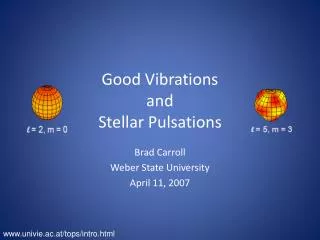
Good Vibrations and Stellar Pulsations. l = 2, m = 0. l = 5, m = 3. Brad Carroll Weber State University April 11, 2007. www.univie.ac.at/tops/intro.html.

E N D
Good VibrationsandStellar Pulsations l = 2, m = 0 l = 5, m = 3 Brad Carroll Weber State University April 11, 2007 www.univie.ac.at/tops/intro.html
In August of 1596, David Fabricius (Lutheran pastorand amateur astronomer) observed o Ceti, a 2nd magnitude star in the constellation Cetus. As it declined in brightness, the star vanished by October. Later it reappeared, and was renamed Mira (“the Wonderful”) By 1660 its 11-month period had been established. The light variations were believed to be caused by “blotches” on the surface of a rotating star. web.njit.edu/~dgary/728/Lecture12.html
In 1784, John Goodricke of York discovered that d Cephei is variable: P = 5 days, 8 hours
d Cephei is the prototype of the Classical Cepheids From Wycombe Astronomical Society, wycombeastro.org.uk/news.shtm magnitude varies from 3.4 to 4.3,so luminosity changes by factor of100(Dm/5) = 100(0.9/5) = 2.3
Edward Charles Pickering’s Computersat Harvard Observatory From left to right: Ida Woods, Evelyn Leland, Florence Cushman, Grace Brooks,Mary Van, Henrietta Leavitt, Mollie O'Reilly, Mabel Gill, Alta Carpenter, Annie Jump Cannon, Dorothy Black, Arville Walker, Frank Hinkely, andProfessor Edward King (1918). www.astrogea.org/surveys/dones_harvard.htm
Henrietta Swan Leavitt (1868 – 1921) Found 2400 Classical Cepheids In 1912, discovered the Period-Luminosity Relation
Cepheids in the SMC From Shapley, Galaxies, Harvard University Press, Cambridge, MA, 1961.
Calibration: The Distance to a Cepheid The nearest Cepheid is Polaris (over 90 pc), too far for trigonometric parallax. d (pc) = 1/p (in arcsec) In 1913, Ejnar Hertzsprung of Denmark used least squares mean parallax to determine the average magnitude M = -2.3 for a Cepheid with P = 6.6 days. d (pc) = 4.16/slope (in arcsec/yr)(4.16 AU/yr is the Sun’s motion) www.cnrt.scsu.edu/~dms/cosmology/DistanceABCs/distance.htm
Period – Luminosity Relation M<V> = -2.81 log10Pd – 1.43 d (pc) = 10(m-M+5)/5 Sandage and Tammann, The Astrophysical Journal, 151, 531, 1968.
How to Find the Distance to aPulsating Star • Find the star’s apparent magnitude m (just by looking) • Measure the star’s period (bright-dim-bright) • Use the Period-Luminosity relation to find the stars absolute magnitude M • Calculate the star’s distance (in parsecs) using d (pc) = 10(m-M+5)/5
What is the Milky Way? antwrp.gsfc.nasa.gov/apod/ap060801.html
Thomas Wright, An Original Theory on New Hypothesis of the Universe, 1750. Kapteyn, The Astrophysical Journal, 55, 302, 1922.
In 1913, Hertzsprung calculated that the distance to the Small Magellanic Cloud was 33,000 light years. This was the greatest distance ever determined for an astronomical object. In 1917, Harlow Shapley used Hertzsprung’s calibration of the period-luminosity relation to determine the distance to the globular clusters (some of which contain Cepheids).
The Milky Way has about 120 globular clusters,each containing perhaps 500,000 stars. One-third of all known globular clusters covers only 2% of the sky, in the constellation Sagittarius. Shapley found the globular clusters had a spherical distribution. homepage.mac.com/kvmagruder/bcp/aster/constellations/Sgr.htm
The Sun was removed from the center of the universe, and placed at an inconspicuous spot near the edge.
The Great Debate: Are the spiral Nebulae (such as M31 = Andromeda) comparable in size with the Milky Way, or are they much smaller and near? Harlow Shapley (left)vsHeber D. Curtis (right) In 1925, Edwin Hubble discovered a Classical Cepheid in M31. Hubble used Hertzsprung’s calibration of the period-luminosity relation to calculate that M31 was over 300,000 pc distant. At this distance, M31 would be 10 kpc in diameter. The spiral nebulae are galaxies like our own.
Classical Cepheids are the standard candles of the universe www.pas.rochester.edu/~afrank/A105/LectureXV/LectureXV.html
Embarrassments! • Our galaxy seemed to be the largest. • The globular clusters in M31 were underluminous by a factor of 4. In 1952, Walter Baade discovered that there are two types of Cepheids and two period – luminosity relations.
Population I Cepheids (Classical Cepheids) are relatively rich in heavy elements. Population II Cepheids (W Virginis stars) are relatively poor in heavy elements. Pop I Cepheids are four times more luminous than Pop II Cepheids.outreach.atnf.csiro.au/education/senior/astrophysics/variable_cepheids.html
So ….. • Hertzspring’s Classical Cepheids (Pop I) were obscured by dust in the plane of the Galaxy, so luminosities of Classical Cepheids were calibrated too low by a factor of 4. • Shapley mistook the Pop II Cepheids in globular clusters for Pop I Cepheids, so his Pop II Cepheids in the globular clusters were properly calibrated (luck!). • Shapley’s distances to the globular clusters were correct. • Hubble’s Pop I Cepheids in M31 were underluminous by a factor of 4, so M31(and all other galaxies measured using Classical Cepheids) was twice as far away as previously believed, and twice as large. • The globular clusters around M31 are as bright as those surrounding our own galaxy.
The Instability Strip on the HR Diagram DT ~ 600 – 1100 K density period incr incr < hotter cooler >
Luminous Blue Variables • Wolf-Rayet stars • Cephei stars • Planetary Nebula Nuclei Variables • Miras, Semi-Regular variables • Slowly Pulsating B stars • DO-type Variable white dwarfs • DB-type Variable white dwarfs • DA-type Variable white dwarfs
Some Pulsating Variables R = radial oscillations NR = nonradial oscillations
RR Lyrae variables in the globular cluster M3 (one night’s observation) cfa-www.harvard.edu/~jhartman/M3_movies.html
Light and radial velocity curves for d Cephei receding approaching Schwarzschild, Harvard College Observatory Circular, 431, 1938
d Cephei radius Schwarzschild, Harvard College Observatory Circular, 431, 1938
Schwarzschild, Harvard College Observatory Circular, 431, 1938
The star is brightest when its surface is moving outward most rapidly, and not at minimum radius – a phase lag. Schwarzschild, Harvard College Observatory Circular, 431, 1938
Consider the adiabatic, radial pulsation of a gas- filled shell. Linearize the equation of motion by setting to get
For adiabatic motion, Also, Set and plug into
The result is or dynamical instability P
for the Sun, P Compare this with the time for sound to cross a star’s diameter: P Estimate! P
The Period – Mean Density Relation density period incr incr
Organ Pipes and Pulsating Stars
Pulsating Stars are Heat Engines The Otto cycle. 1. In the exhaust stroke, the piston expels the burned air-gas mixture left over from the preceding cycle. 2. In the intake stroke, the piston sucks in fresh air-gas mixture. 3. In the compression stroke, the piston compresses the mixture, and heats it. 4. At the beginning of the power stroke, the spark plug fires, causing the air-gas mixture to burn explosively and heat up much more. The heated mixture expands, and does a large amount of positive mechanical work on the piston. www.lightandmatter.com/html_books/0sn/ch05/ch05.html
In 1918, Arthur Stanley Eddington proposed that pulsating stars are heat engines, transforming thermal energy into mechanical energy. He proposed two mechanisms: • Energy MechanismEddington suggested that when the star is compressed, more energy is generated by sources in the stellar core. Ineffective. The core pulsation amplitude is very small. • Valve Mechanism“Suppose that the cylinder of the engine leaks heat and that the leakage is made good by a steady supply of heat. The ordinary method of setting the engine going is to vary the supply of heat, increasing it during compression and diminishing it during expansion. That is the first alternative we considered. But it would come to the same thing if we varied the leak, stopping the leak during compression and increasing it during expansion. To apply this method we must make the star more heat-tight when compressed than when expanded; in other words, the opacity must increase upon compression.”
But this does not work for most stellar material! Why? The opacity is more sensitive to the temperature than to the density, so the opacity usually decreases with compression (heat leaks out). But in a partial ionization zone, the energy of compression ionizes the stellar material rather than raising its temperature! In a partial ionization zone, the opacity usually increases with compression! Partial ionization zones are the direct cause of stellar pulsation.
hydrogen ionization zone (H H+ and He He+) T = (1 – 1.5) x 104 K • helium II ionization zone (He+ He++) T = 4 x 10⁴ K C C If the star is too hot, the ionization zones will be too near the surface to drive the oscillations. This accounts for the “blue edge” of the instability strip. The “red edge” is probably due to the onset of convection. f u n d a m e n t a l 1 s t o v e r t o n e n o p u l s a t I o n
Phase lag problem: A Cepheid is brightest when its surface is moving outward most rapidly, and not at minimum radius – a phase lag. • the emergent luminosity varies inversely with the mass lying above the hydrogen ionization zone • the luminosity on the bottom of the hydrogen ionization zone is largest at minimum radius • the hydrogen ionization zone is moving outwards (through mass) fastest at minimum radius • the hydrogen ionization is farthest out ~ ¼ cycle later • the luminosity peaks ~ ¼ cycle after minimum radius
Nonradial Oscillations Pulsational corrections df to equilibrium model scalar quantities f0 go as (the real part of) l = 0 radial m > 0 retrograde m < 0 prograde m = 0 standing click here http://gong.nso.edu/gallery/images/harmonics
Smith, The Astrophysical Journal, 240, 149, 1980 to Earth In a rotating star, frequencies are rotationally split (~ Zeeman). Si III l = 2, m = 0, -1, -2
Two Types of Nonradial Modes www.astro.uwo.ca/~jlandstr/planets/webfigs/earth/slide1.html
Two Types of Frequencies The acoustic frequency: The Brunt-V@is@l@ (buoyancy) frequency:
or l = 2
p modes a surface gravity wave