Download
1 / 11
110 likes | 382 Vues
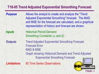
Section 7.2: Exponential Smoothing. Quantitative Decision Making 7 th ed By Lapin and Whisler. Simple Exponential Smoothing. Graphing Actual vs Forecast Values. Forecasting Errors. Two Parameter Smoothing. Simple Exponential Smoothing. Compute T 3. Compute b 3.

E N D
Section 7.2: Exponential Smoothing Quantitative Decision Making 7th ed By Lapin and Whisler
Seasonal Exponential Smoothing with Three Parameters • Many time series have regular seasonal patterns to be incorporated into forecasts. • The three-parameter model incorporates a seasonal smoothing constant b (beta): Tt = a(Yt /St –p) + (1 – a)(Tt –1 + bt –1) bt = g(Tt– Tt –1) + (1 – g)bt –1 St = b(Yt /Tt) + (1 – b)St –p Ft+1 = (Tt + bt) St –p+1
Forecasting withThree Parameters • The above works for p = 4 quarters or p = 12 months. • The preceding slide needs 6 quarters to generate the first (very bad) forecast. • The process settles quickly, providing good forecasts p periods into the future.