Download
1 / 36
360 likes | 497 Vues
Showcase of a Biome-BGC workflow presentation. Zoltán BARCZA. Training Workshop for Ecosystem Modelling studies Budapest, 29-30 May 2014. Biome-BGC Typical process-based biogeochemical model to simulate plant growth with full accounting on carbon, nitrogen and water flows.

E N D
Showcase of a Biome-BGC workflow presentation Zoltán BARCZA Training Workshop for Ecosystem Modelling studies Budapest, 29-30 May 2014
Biome-BGC • Typical process-based biogeochemical model to simulate plant growth with full accounting on carbon, nitrogen and water flows. • Due to the complex nature of plant growth and mortality and their drivers large uncertainties exist in • model structure – caused by many simplifications and assumptions • parameterization – plant traits change from point to point • driving environmental variables – meteorology, soil, topography… • magnitude and nature of human intervention
Role of measurement data Measurements: we can ‘train’ the model to perform better [=calibration] PROBLEM: state-of-the-art models are highly complex and non-linear so common sense [tuning model parameters manually] does not work anymore SOLUTION: statistical calibration; all parameters are changed simultaneously, and we use mathematical statistics to evaluate the model against data [GLUE, Bayesian calibration, etc.] PROBLEM AGAIN: if model structure has errors, can we trust the calibrated parameters? Not really….
Biome-BGC within BioVeL • - development of Biome-BGC, current BioVeL-supported version is Biome-BGC MuSo v2.2.1 • major improvements: implementation of human intervention, major improvement in soil hydrology and herbaceous vegetation phenology [+ other small details (“Devil lives in details”)] • continuous development = continuous optimization!
Biome-BGC: plant function type logic PFT: classification of plants based on basic traits like leaf longevity and woody/non-woody characteristics But what about the PFT logic?
Model parameter estimation (calibration) • - GLUE method (based on Monte-Carlo method) • Bayesian calibration (Monte-Carlo method with Metropolis algorithm) • Levenberg-Marquardt • Kalman filter • genetic algorithm… + many other • The result is optimized parameters + uncertainty intervals for parameters (a posteriori distribution). Additionally, confidence interval can be estimated for the prognostic run
Basics of calibration As we have both reference data (measurement) and simulated data (Biome-BGC) for the same variable (e.g. GPP, Reco), we can compare them and judge the quality of the simulation. Question: how can we say which simulation is better than another?
1 2
mean of model and measurement: BIAS of MODEL1: -2.1 BIAS of MODEL2: 0!!!
Message There are different metrics to quantify measurement-model agreement/mismatch. We should choose one objective function that fits our needs. Example: use RMSE to quantify the bias
If misfit is higher, simulation is worse. So we need to minimize misfit to get good simulation. The usual statistical expression of model goodness is likelihood, e.g.:
There are many likelihood definitions in the literature. Hidy et al., 2012:
Further problems: multi-objective calibration Monitoring of carbon balance components usually involve measurement of different components [e.g. stem and root biomass, litter, NEE, H2O flux…]. It would be nice to optimize the model taking into account more than one data stream. This is possible – the question is once again: how should we construct model-measurement misfit (objective function).
BioVeL approach Example for using eddy-covariance data to optimize Biome-BGC MuSo individual cost functions
BioVeL approach aggregate multi-objective cost function [Keenan et al. 2011 Oecologia] Aggregate likelihood The datastreams are equally important!
MACSUR is a knowledge hub within FACCE-JPI (Joint Programming Initiative for Agriculture, Climate Change, and Food Security). MACSUR gathers the excellence of existing research in livestock, crop, and trade science to describe how climate variability and change will affect regional farming systems and food production in Europe in the near and the far future and the associated risks and opportunities for European food security.
MACSUR • Biome-BGC MuSo participates in Grassland model intercomparison [part of LiveM theme, grassland and livestock modelling] • TASKS: • blind tests [previously calibrated models are run using driving data and management] • calibrated runs [participants has to re-calibrate their models using information from data-rich sites (eddy-covariance sites)]
CALIBRATION • It would not have been possible without BioVeL infrastructure! • Monte-Carlo experiment was used • post-processing was performed using IDL • post-processing was the testbed for the workflow representation [GLUE]
CALIBRATION MCE settings EPC MuSo 2.2 #row number min max description [optional] 13 0.01 0.2 (1/yr) annual whole-plant mortality fraction 15 0.5 2.5 (ratio) (ALLOCATION) new fine root C : new leaf 20 0.1 0.9 (prop.) (ALLOCATION) current growth proportion 21 14.0 44.0 (kgC/kgN) C:N of leaves 39 0.7 1. (DIM) canopy light extinction coefficient 41 30.0 80.0 (m2/kgC) canopy average specific leaf area 43 0.1 0.3 (DIM) fraction of leaf N in Rubisco 45 0.001 0.006 (m/s) maximum stomatal conductance EPC_END INI 34 0.3 1.5 (m) maximum root depth 42 0.001 0.003 (kgN/m2/yr) symbiotic+asymbiotic fixation of N INI_END Guidance: White et al. 2000 (typically)
CALIBRATION GLUE was used to visualize and post-process the results. What is GLUE? General Likelihood Uncertainty Estimation
Oensingen 0. maximum root depth 1. symbiotic+asymbiotic fixation of N 2. annual whole-plant mortality fraction 3. new fine root C : new leaf 4. current growth proportion 5. C:N of leaves 6. canopy light extinction coeff 7. canopy average specific leaf area 8. fraction of leaf N in Rubisco 9. maximum stomatal conductance
Laqueuille-intensive 0. maximum root depth 1. symbiotic+asymbiotic fixation of N 2. annual whole-plant mortality fraction 3. new fine root C : new leaf 4. current growth proportion 5. C:N of leaves 6. canopy light extinction coeff 7. canopy average specific leaf area 8. fraction of leaf N in Rubisco 9. maximum stomatal conductance
Monte-Bodone 0. maximum root depth 1. symbiotic+asymbiotic fixation of N 2. annual whole-plant mortality fraction 3. new fine root C : new leaf 4. current growth proportion 5. C:N of leaves 6. canopy light extinction coeff 7. canopy average specific leaf area 8. fraction of leaf N in Rubisco 9. maximum stomatal conductance