Alternation
Giorgi Japaridze Theory of Computability. Alternation. Section 10.3. 10.3.a. Giorgi Japaridze Theory of Computability. Alternating Turing machines. Definition 10.16 An alternating Turing machine is a nondeterministic TM with an additional

Alternation
E N D
Presentation Transcript
Giorgi Japaridze Theory of Computability Alternation Section 10.3
10.3.a Giorgi JaparidzeTheory of Computability Alternating Turing machines Definition 10.16 An alternating Turing machine is a nondeterministic TM with an additional feature. Its states, except for the accept and reject states, are divided into universal states and existential states. When we run an alternating TM on an input string, we label each node of its nondeterministic computation tree with∧ or ∨, depending on whether the corresponding configuration contains a universal or existential state. We determine acceptance by designating a node to be accepting if it is labeled with ∧and all of its children are accepting or if it is labeled with∨ and at least one of its children is accepting. ∨ ∨ ∨ ∨ ∨ ∧ ∨ ∧ ∨ reject ∨ ∨ reject ∨ ∨ ∨ reject reject accept reject reject accept nondeterministic computation tree alternating computation tree
10.3.b Giorgi JaparidzeTheory of Computability ATIME and ASPACE defined ATIME(t(n)) =def {L | L is decided by an O(t(n)) time alternating TM} ASPACE(t(n)) =def {L | L is decided by an O(t(n)) space alternating TM} We further define AP, APSPACE and AL to be the classes of languages that are decided by alternating polynomial time, alternating polynomial space, and alternating logarithmic space TMs, respectively. Example 10.19 Here is an alternating polynomial time algorithm for the UNSATISFIABILITY problem for Boolean formulas: “On input <>: 1. Universally select all assignments to the variables of . 2. For a particular assignment, evaluate . 3. If evaluates to 0, accept; otherwise reject.”
10.3.c Giorgi JaparidzeTheory of Computability MIN-FORMULA is in AP Example 10.20 This example features a language in AP that isn’t known to be in NP or coNP. Two Boolean formulas are said to be equivalent iff they evaluate to the same value on all assignments to their variables. A minimal formula is one that has no shorter equivalent. Let MIN-FORMULA = { <> | is a minimal Boolean formula}. The following is an alternating polynomial time algorithm for this language. “On input <>: 1. Universally select a formula that is shorter than . 2. Existentially select an assignment to all relevant variables. 3. Evaluate both and on this assignment. 4. Accept if the formulas evaluate to different values. Reject otherwise.”
10.3.d Giorgi JaparidzeTheory of Computability Main theorems Theorem 10.21 a) For f(n) ≥ n we have ATIME(f(n)) SPACE(f(n)) ATIME(f2(n)) . b) For f(n) ≥ log n we have ASPACE(f(n)) = TIME(2O(f(n))). Corollary AL = P AP = PSPACE APSPACE = EXPTIME
10.3.e Giorgi JaparidzeTheory of Computability Alternating machines provide a way to define a natural hierarchy of problems within the class PSPACE. The polynomial time hierarchy Definition 10.27 Let i be a natural number. A i-alternating TM is an alternating TM that contains at most i runs of universal or existential steps, starting with existential steps. A i-alternating TM is similar except that it starts with universal steps. iTIME(f(n)) is defined as the class of languages that a i-alternating TM can decide in O(f(n)) time. Similarly for iTIME(f(n)). Similarly for iSPACE(f(n)) and iSPACE(f(n)). The polynomial time hierarchy is the collection of classes iP = iTIME(nk) and iP = iTIME(nk) k k PH is defined as iP, which can be seen to be the same as iP. i i Clearly NP =1P and coNP = 1P. Also, MIN-FORMULA 2P.