Decision Making, Systems, Modeling, and Support

1. Decision Making, Systems, Modeling, and Support

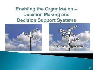
2. Slide 2- 1 2.1 Introduction and Definition • See the vignette story. A typical business decision: • The decision may be made by a group • There are several, possibly contradictory objectives • There could be hundreds or even thousands of alternatives to consider • The results of making a decision today will sometimes materialized in the future. No one is a perfect predictor of the future. Especially in the long run. • Many decisions involve risk, different people have different attitudes toward risk • Decision makers are interested in what-if scenarios

3. Slide 2- 2 2.1 Introduction and Definition • Experimentation with the real system (that is, investing and seeing what will happen) meaning trial-and-error, may results in a loss. • Experimentation with the real system is possible only for one set of conditions • Changes in the decision-making environment can occur continuously. So how are decisions made by serious investors? To answer this question, one must first understand the process and the important issues of decision making. Then one can understand the methodologies that have been developed to assist decision makers and the role that information systems can play in supporting decision making. These topics are addressed in this chapter.

4. Slide 2 - 3 2.1 Introduction and Definition • Decision Making • Decision making is a process of choosing among alternative courses of action for the purpose of attaining a goal or goals. According to Herbert A. Simon (1977), Managerial decision making is synonymous with the the whole process of management. To illustrate the idea, consider the important managerial functions of planning. Planning involves a series of decisions: What should be done? When? How? Where? And by Whom? (5W) Hence, planning implies decision making. Other functions in the management process, such as organizing and controlling, also involve making decisions.

5. Slide 2 - 4 2.1 Introduction and Definition • Decision Making and Problem Solving A problem occurs when 1) a system does not meet its established goals, 2) does not yield the predicted results, or 3) does not operate as initially intended. Problem solving is not only the solution of trouble areas but also the investigation of opportunities. Understanding the terms decision-making and problem solving can be very confusing. One way to distinguish between them is to examine the phases of the decision process. These phases are (1) intelligence, (2) design, (3) choice, and (4) implementation. One school of thought considers the entire process (steps 1-4 ) as problem solving, and the choice step is considered decision making.

6. Slide 2 - 5 2.1 Introduction and Definition Decision Making and Problem Solving (Continued) Another view is that steps 1-3 constitute decision making that ends with a recommendation whereas problem solving additionally includes the actual implementation of the recommendation (step 4). We use the terms decision making and problem solving interchangeably. One more view is the three stages of decision making-intelligence, design, and choice---are augmented by implementation and monitoring to results in problem solving.

7. Slide 2 - 6 2.2 Systems The acronyms DSS, GDSS, EIS, and ES include the term systems. A system is a collection of objects such as people, resource, concepts, and procedures intended to perform an identifiable function or to serve a goal. For example, an university is a system of students, faculty, staff, administrators, buildings, equipment, ideas, and rules with the goal of educating students, producing research, and providing service to the community (which is another system). A clear definition of the goal function is a critical consideration in MSS design. For instance, the purpose of an air defense system is to protect ground targets, not just to destroy attacking aircraft or missiles.

8. Slide 2 -7 2.2 Systems The notion of levels (or a hierarchy) of systems reflect that all systems are actually subsystems because all are contained within some larger system. For example, a bank includes such subsystems as the commercial loan department, the consumer loan department, the savings department, and the operations department. The bank itself may also be a subsidiary of a holding corporation, such as the Bank of America, which is a subsystem of the California banking system, which is a part of the national banking system, which is a part of the national economy, and so on. The interconnections and interactions among the subsystems are called interfaces.

9. Slide 2 -8 2.2 Systems The System and Its Environment Environment Customers Weather Condition Government Inputs Processes Outputs Performances Conseq. Finished goods Services Delivered Procedures Programs Tools Activities Decisions Raw Materials Costs Resources Vendors Feedback Decision Maker Competition System Boundary Banks Stockholders

10. Slide 2 -9 2.2 Systems The Structure of a System Systems are divided into three distinct parts: inputs, process, and outputs. They are surrounded by an environment and often include a feedback mechanism. In addition, a human decision maker is considered to be part of the system. • Inputs Inputs are elements that enter the system. Examples of inputs are raw materials entering a chemical plant, patients admitted to a hospital, or data input into a computer. • Processes Processes are all the elements necessary to convert or

11. Slide 2 - 10 2.2 Systems transform the inputs into outputs. For example, a process in a chemical plant may include heating the material, using operating procedures, using a material handling subsystems, and using employees and machines. In a hospital, a process may include conducting tests and performing a surgery. In a computer, a process may include activating commands, executing computations, and storing information. Outputs Outputs are the finished products or the consequences of being in the system. For example, fertilizers are some output of a chemical plant, cured people are an output of a hospital, and reports may be the outputs of a computer system.

12. Slide 2 - 11 2.2 Systems • Feedback There is a flow of information from the output component to the decision maker concerning the system’s output or performance. Based on this information the decision maker, who acts as a control, may decide to modify the inputs or the processes, or both. This flow, which appears as a closed loop, is called feedback. • The Environment The environment of the system is composed of several elements that lie outside it in the sense that they are not inputs, outputs, or processes. However, they affect the system’s performance and consequently the attainment of its goals, One way to identify the elements of the environment is by answering two

13. Slide 2 - 12 2.2 Systems two questions as suggested by Churchman (1975). • Does the element matter relative to the system’s goals? • Is it possible for the decision maker to significantly manipulate this element? If and only if the answer to the first question is yes, but the answer to the second is no, should the element be considered part of the environment. Environmental elements can be social, political, legal, physical, and economical. Often they consist of other systems. For example, in a chemical plant, the suppliers, competitors, and customers are elements of the environment.

14. Slide 2 - 13 2.2 Systems In a decision support system of the company, a telecommunications network, and the personal department may be some elements of the environment. • The Boundary A system is separated from its environment by a boundary. The system is inside the boundary, whereas the environment lies outside. Boundaries may be physical (for example, the system is a department in Building C), or the boundary may be some nonphysical factors. For example, a system can be bounded by time. In such a case, we may analyze an organization for a period of only 1 year. When studying systems, it is often necessary to arbitrarily define the boundaries to narrow the scope of the system and simplify its analysis. Such boundaries are related to the concepts of closed and open systems.

15. Slide 2 - 14 2.2 Systems • Close and Open System A close system is at one extreme along a continuum that reflects the degree of independence of systems (the open system is at the other extreme). A closed system is totally independent, whereas an open system is very dependent on its environment and may deliver outputs into the environment. When determining the impact of decisions on an open system, we must determine its relationship with the environment and with related systems. In a closed system, it is not necessary to do this because the system is considered to be isolated. Many computer systems, such as transaction processing systems (TPS), are considered closed systems.

16. Slide 2 - 15 2.2 Systems A special type of closed system is called the black box, in which inputs and outputs are well defined, but the process itself it not specified. Many managers like to treat computer systems as black boxes; in other words, they are not concerned with how the computer works. They think of it like a telephone or an elevator. They simply use these devices independent of the operational details. DSSs attempt to deal with systems that are fairly open. Such systems are complex, and during their analysis, one must determine the impacts on and from the environment. To illustrate the difference between a DSS and a fundamental Management Science approach, consider the two inventory systems outlined in the following table.

17. Slide 2 -16 2.2 Systems Management Science, Inventory DSS Factors EOQ (closed systems) (open systems) Demand Constant Variable, influenced by Many factors Unit cost Constant May change daily Lead time Constant Variable, difficult to predict Vendors and users Excluded from analysis Maybe included to predict Weather and other Ignored May influence demand and lead environmental factors time

18. Slide 2 -17 2.2 Systems • An Information System Systems are evaluated and analyzed with two major classes of performance measures: Effectiveness and Efficiency. Effectiveness is the degree to which goals are achieved. It is therefore concerned with the results or the outputs of a system (such as total sales or earnings per share) Efficiency is a measure of the use inputs (or resources) to achieve outputs (for examples, how much money is used to generate a certain level of sales). Peter Drucker proposed an interesting way to distinguish between the two terms: Effectiveness is doing the right thing. Efficiency is doing the thing right.

19. Slide 2 -18 2.2 Systems • An important characteristic of MSS is their emphasis on the effectiveness, or “goodness”, of the decision produced, rather than on the computational efficiency, which is usually a major concern of a TPS. • In many managerial systems, and especially those involving the delivery of human service (such as education, health, or recreation), measurement of the system’s effectiveness and efficiency is a major problem. This is because of several, often non-quantifiable, conflicting goals.

20. Slide 2 -19 2.3 Models • A major characteristic of decision support systems is the inclusion of at least one model. The basic idea is to perform the DSS analysis on a model of reality rather than on the real system itself. • A model is a simplified representation or abstraction of reality. It is usually simplified because reality is too complex to copy exactly and because much of the complexity is actually irrelevant in solving the specific problem. • The representation of systems or problems by models can be done with various degree of abstraction; therefore, models are classified into three groups according to their degree of abstraction: Iconic/Symbolic, Analog, and Mathematical.

21. Slide 2 -20 2.3 Models • Iconic (Scale) Models An iconic model—the least abstract model—is a physical replica of a system, usually on a different scale from the original. Iconic models may appear in three dimensions, such as that of an airplane, car, bridge, or production line. Photographs are another type of iconic scale model, but on only two dimensions. Graphics user interfaces and object-oriented programming are other examples of the use of icons. • Analog Models An analog model is more abstract than an iconic model and is a symbolic representation of reality. These are usually two-dimensional charts or diagrams; they could be physical models, but the shape of the model differs from that of the actual systems. Some examples include:

22. Slide 2 -21 2.3 Models • Analog Models • Organization charts that depict structure, authority, and responsibility relationships • A map in which different colors represent objects such as bodies of water or mountains • Stock market charts that represent the price movements of stocks. • Blueprints of a machine or a house • A speedometer • A thermometer

23. Slide 2 -22 2.3 Models • Mathematical (Quantitative ) Models The complexity of relationships in many organizational systems cannot be represented with icons or analogically, or such presentation may be cumbersome and time-consuming to use. Therefore, more abstract models are described mathematically. Most DSS analyses are performed numerically with mathematical or other quantitative model. • The Benefits of Model • Models enable the compression of time. Years of operations can be simulated in minutes or seconds of computer time.

24. Slide 2 -23 2.3 Models • The Benefits of Model (continued) • Model manipulation (changing decision variables or the the environment) is much easier than manipulating the real system. Experimentation is therefore easier to conduct and does not interfere with the daily operation of the organization. • The cost of modeling analysis is much less than the cost of a similar experiment conducted on a real system • The cost of making mistakes during a trial-and-error experiment is much less when models are used rather than real systems. • Today’s environment involves considerable uncertainty. With modeling, a manager can calculate the risks involved in specific actions.

25. Slide 2 -24 2.3 Models • The Benefits of Model (continued) • The use of mathematical models enables the analysis of a very large, sometimes infinites number of possible solutions. With today’s advanced technology and communications, managers often have a large number of alternatives from which to choose. • Models enhance and reinforce learning and training. Note that recent advances in computer graphics have lead to an increased tendency to use iconic and analog models to complement MSS mathematical modeling. For ex. Visual Simulation.

26. Slide 2 -25 2.4 The Modeling Process: A Preview Example: How much to Order? The Ma-Pa Grocery is a small neighborhood food store on the west side of New York City. Bob and Jan, the owners, are very sensitive to their clients’ wishes. They also are concerned with the financial viability of the store. A major product they sell is bread. Bread causes them headaches. Some days, there is not enough bread; other days, bread is overstocked so they have to sell it the next day at a loss. Their problem is, How much bread to stock each day? Bob and Jan apply the following solution approaches to the problem. • Trial-and-Error with Real System • In this approach, the owners try to learn from experimentation on the real system. Namely, they change the quantities of bread stocked and observed what

27. Slide 2 -26 2.4 The Modeling Process: A Preview • happens. If they find they are short on bread too often, they will increase the quantities ordered. If they find what too much bread is left, they will decrease the quantities ordered. Sooner or later they will figure out how much bread to order. • Although this approach may be very successful for Bob and Jan, it may fail in many other cases. Trial-and-Error may not work if one or more following conditions exists: • There is too many alternatives (trials) to explore • The cost of making error (part of the trial-and-error approach) is very high • The environment keeps changing. Therefore, learning from experience is difficult or even impossible.

28. Slide 2 -27 2.4 The Modeling Process: A Preview By the time you have experimented with all the alternatives, the environmental conditions will have changed and you have a whole new ball game. Fortunately, there is other approaches to resolve the problem, that is a modeling approach. • Simulation In this case, Jan and Bob play a make-believe game. They ask themselves, “if we order 300 loaves of bread, what will the results be?” The results will depend on the demand, which may be constant or may vary (be stochastic). Simulation, which is based on historical and projected data, can deal with both situations. The model that represents the Ma-Pa Grocery is used to calculate results such as total profits (or loss), percentage of unsatisfied customers, and amount of the leftovers. A big advantage of simulation

29. Slide 2 -28 2.4 The Modeling Process: A Preview modeling is that months of operations can be simulated in seconds if a computer is used. Next, Jan and Bob change the order quantities to 350, 400, 200, 250, and so on. They “run the store” on a computer several times with each daily order quantities over several months, and calculate the results. Finally, they compare the results of each order quantities and decide how much to order. The problem with the simulation approach is that once the experiment is completed, there is no guarantee that the selected daily stocking level is the best (optimal) one. It will be the best of all levels tested, but it is possible that a true best level (the optimal one) is 675, a level not tried. Another problem with the simulation is that Jan and Bob may need professional help to design the simulation study, program it

30. Slide 2 -29 2.4 The Modeling Process: A Preview on a computer, and interpret the statistical results. The cost of creating and testing the model may not be justified. • Optimization A more sophisticated approach to solving the problem is to use an optimization model. Ideally, such a model will generate an optimal (best) order level in seconds. For structured situations, there is very inexpensive and user-friendly software to conduct such an analysis. The limitation of optimization is that it works only if the problem is structured and for most part, deterministic. Specifically, such a model will specify the required input data, the desired output, and the mathematical relationship in a precise manner. Obviously, if the reality differs significantly from the model, optimization cannot be used.

31. Slide 2 -30 2.4 The Modeling Process: A Preview • Optimization Recall that DSS deals with unstructured problems. Does this preclude optimization? Not necessarily. Many times it is possible to break a problem into sub-problems, some of which are structured enough to justify applying optimization. Also optimization can be combined with simulation for the solution of complex problems. • Heuristics Jan and Bob can use some general rules. For example, they can stock today the average daily quantity demanded over the last seven days. Another rule that they can use is to stock each day the quantity demanded on the same day one week earlier. The rules may be provided by experts or even derived by trial-and-error.

32. Slide 2 -31 2.4 The Modeling Process: A Preview • The decision-making Process To better understand modeling, it is advisable to following a systematic decision making process, which, according to Simon (1977), involves three major phases: intelligence, design, and choice. A fourth phase, implementation, was added later. A conceptual picture of the decision-making process is shown in the following figure. See next slide.

33. Slide 2 -32 Organizational Objectives Search and scanning procedures Data Collection Problem Identification Problem ownership Problem classification Problem statement Simplification Reality Intell. Phase Assumption Problem Statement Formulate a model Set criteria for choice Search for alternatives Predict and measure outcomes Validation of the model Design Phase Success Alternatives Verification, Testing of proposed solution Solution to the model Sensitivity Analysis Selection of best alternatives Plan for implementation Choice Phase Imp. Of solution Solution Failure

34. Slide 2 -33 2.5 The Intelligence Phase Intelligence entails scanning the environment, either intermittently or continuously. It includes several activities aimed at identifying problem situations or opportunities. • Find the problem The intelligence phase begins with the identification of organizational goals and objectives and determination of whether they are being met. In this phase, one attempts to • Determine whether a problem exists • Identify its symptoms • Determine its magnitude, and • Explicitly define the problem However, the relationship between the symptoms and the real problem is difficult to distinguish. At the same time, the collection data and the estimation of future data are among the most difficult steps. Because:

35. Slide 2 -34 2.5 The Intelligence Phase • Outcomes may occur over an extended period of time. As a results, revenues, expenses, and profits will be recorded at different points in time. To overcome this difficulty, the present-value approach should be used, if the results are quantifiable. • It is often necessary to use a subjective approach to data estimation • It is assumed that future data will be similar to historical data. If not, it is necessary to predict the nature of the change and include it in the analysis. Once the preliminary investigation is completed, it is possible to determine whether a problem really exists, where it is located, and how significant it is. • Problem Classification

36. Slide 2 -35 2.5 The Intelligence Phase • Problem Classification This activity is the conceptualization of a problem in an attempt to classify it into a definable category. An important classification is according to the degree structuredness evident in the problem. Simon (1977) has distinguished two extreme situations regarding structuredness of decision problems. • Programmed problems • Nonprogrammed problem • Problem Decomposition Many complex problems can be divided into sub-problems. Solving the simpler subproblems may help in solving the complex problems. Also, some seemly poorly structured problems may have some highly structured subproblems. Such an approach also facilitates communication between the people involved in the solution.

37. Slide 2 -36 2.5 The Intelligence Phase • Problem Ownership In this phase, it is important to establish the ownership problem. A problem exists in an organization only if someone or some group is willing to take the responsibility to solve it and if the organization has the capability to solve it. For example, interest rates. Many companies feel that they have a problem because interest rates are too high. Because the IR levels are determined at the national level and most companies can not do any thing about them, high IR are the problem of the federal government, not of a specific company. The problem companies face is how to operate in an environment in which the IR is high. The intelligence phase ends with a problem statement. At that time, the design phase can be started.

38. Slide 2 -37 2.6 The Design Phase • The design phase involves generating, developing, and analyzing possible courses of action. This includes activities such as understanding the problem and testing solutions for feasibility. Also, in this phase, a model of the problem situation is constructed, tested, and validated. • Modeling involves the problem abstracted into quantitative and/or qualitative forms. • For the math model, the variables are identified and the equations describing their relationships are established. • The tasks of modeling involves a combination of art and science. We present the following topics of modeling as they relate to quantitative models.

39. Slide 2 -38 2.6 The Design Phase • The components of the model • The structure of the model • Selection of a principle of choice • Developing alternatives • Predicting outcomes • Measuring outcomes • Scenario • The Components of Quantitative Models All models are made up of three basic components (see figure 2.3): decision variables, uncontrollable variables, (and/or parameters), and results (outcome) variables. These components are connected by mathematical relationships. In a non-quantitative model, the relationships are symbolic or qualitative. The results of decisions are determined by the decision made (value of the decision variables),the factors that are uncontrollable by the decision makers, and the relationships among variables.

40. Slide 2 -39 2.6 The Design Phase • Results variables Results variables reflect the level of effectiveness of the system; that is, they indicate how well the system performance or attains its goals. • Decision Variables Decision variable describe the alternative course of action. The values of these variables are determined by the decision maker. • Uncontrollable variables or parameters In any decision situation, there are factors that affect the results variables but are not under the control of the decision maker. These factors can be either fixed, in which case they called parameters, or they can vary (variables). Examples are interest rates, a city’s building code, tax regulations and prices of utility. Some of these variables places limits on the decision maker and therefore form what are called the

41. Slide 2 -40 2.6 The Design Phase constraints of the problem. • Intermediate Results of Variables Reflect intermediate outcomes. The general structure of a Quantitative model Uncontrollable Variables Results Variables Decision Variables Mathematical Relationships

42. Slide 2 -41 2.6 The Design Phase Area DV RV UV and P Financial Invest. Alternatives Total Profit Inflation Rate Investment and amount Rate of Return(ROR) Prime Rate How long to invest Earning per share Competition When to invest Liquidity level Marketing Advertising budget Market share Customer’s income Where to advertise Customer Competitor’s satisfaction action Manufacturing What & How much to Total cost Machine capacity Inventor Levels Quality Level Technology Compensation Employee Material Price Programs Satisfaction Accounting Use of computers Data Processing cost Computer Tech. Audit schedule Error rate Tax rates Legal requirement Transportation Shipment schedule Total Trport cost Delivery dist.

43. Slide 2 -42 2.6 The Design Phase Area DV RV UV and P Transportation Shipment schedule Total Trport cost Delivery dist. Regulations Service Staffing levels Customer satisfaction Demand for svce. • The structure of Quantitative Models The components of a quantitative model are connected by sets of mathematical expressions such as equations or inequalities. Example: The product-mix model. MBI Corporation makes special-purpose computers. A decision must be made: How many computers must be produced next month in Boston plant?

44. Slide 2 -43 2.6 The Design Phase Two types of computers considered: the CC-7, which requires 300 days of labor and $10,000 in materials, and the CC-8, which requires 500 days of labor and $15,000 materials. The profit contribution of each CC-7 is $8,000, whereas that of each CC-8 is $12,000. Currently, the plant has a capacity of 200,000 working days per month, and the material budget is $8,000,000 per month. Marketing requires that at least 100 units of the CC-7 be produced each month and at least 200 units of the CC-8 be produced. The problem is to determine how many units of the CC-7 and how many units of the CC-8 to produce each month to maximize the company’s profits. Modeling. A standard mathematical modeling technique called linear programming is applicable. It has three components: Decision Variables: x1= Units of CC-7 to be produced,

45. Slide 2 -44 2.6 The Design Phase Decision Variables: x1= Units of CC-7 to be produced, x2= Units of CC-8. Results Variables: The total profit = Z. The Objective is to maximize total profit Z = 8,000x1+12,000x2 Uncontrollable variables (constraints) Labor constraint: 300x1+500x2  200,000 (in days) Budget constraint: 10,000x1+15,000x2  8,000,000 (in $) Marketing requirement for CC-7: x1  100 (in units) Marketing requirement for CC-8: x2  200 (in units) This information is summarized in Figure 2.4.

46. Slide 2 -45 2.6 The Design Phase Decision Variables Mathematical (logical) relationship Results Variables x1= units of CC-7 x2 = units of CC-8 Maximize Z (Profit) Subject to constraints Total profit =Z Z=8000x1+12000x2 Uncontrollable variables (constraints) 300x1+500x2  200,000 10,000x1+15,000x2  8,000,000 x1 >= 100 x2 >= 200

47. Slide 2 -46 2.6 The Design Phase Solution: The solution to this problem (derived by a computer) is x1= 333.33, and x2 = 200, Profit = $5,066,667. • Selection of a Principle of Choice • A principle of choice is a decision regarding the acceptability of a solution approach. Are we willing to assume high risk or do we prefer a low-risk approach? • Are we attempting to optimize or satisfy? Of the various principles of choice, two are of prime interest; normative and descriptive.

48. Slide 2 -47 2.6 The Design Phase • Normative Models Normative implies that the chosen alternative is demonstrably the best of all possible alternatives. To find it, one should examine all alternatives and prove that the one selected as indeed the best. This process is basically that of optimization. In operational terms, optimization can be achieved in one of three ways: • Get the highest level of goal attainment from a given set of resources. For example, which alternative will yield the maximum profit from an investment of $1,000,000? (Goal Seeking) • Find the alternative with the highest ratio of goal attainment to cost (for example, profit per dollar investment), or maximize productivity.(sensitivity analysis)

49. Slide 2 -48 2.6 The Design Phase III. Find the alternative with the lowest cost (or other resource) that will fulfill a required level of goals. For example, if your risk is to build a product to certain specifications, which method will accomplish this goal with the least cost? Normative decision theory is based on the following assumptions related to rational decision makers: • Humans are economic beings whose objective is to maximize the attainment of goals; that is, the decision maker is rational • In a given decision situation, all viable alternative course of action and their consequences, or at least the probability and the values of the consequences, are known. • Decision makers have an order or preference that enables them to rank the desirability of all consequences of the analysis.

50. Slide 2 -49 2.6 The Design Phase Optimization models: • Assignment ( best matching of objects) • Dynamic Programming • Goal programming • Investment (maximizing rate of return) • Linear programming • Network models for planning and scheduling • Nonlinear programming • Replacement( capital budgeting) • Simple inventory models (such as EOQ) • Transportation (minimize cost of shipment) Suboptimization: By definition, optimization requires the decision maker to consider the impact of each alternative course of action