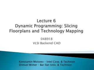
Lecture 6 Dynamic Programming: Slicing Floorplans and Technology Mapping
510 likes | 700 Vues
Lecture 6 Dynamic Programming: Slicing Floorplans and Technology Mapping. 048918 VLSI Backend CAD. Konstantin Moiseev – Intel Corp. & Technion Shmuel Wimer – Bar Ilan Univ. & Technion. Course outline. VLSI design flow overview Introduction to algorithms and optimization

Lecture 6 Dynamic Programming: Slicing Floorplans and Technology Mapping
E N D
Presentation Transcript
Lecture 6Dynamic Programming: Slicing Floorplans and Technology Mapping 048918 VLSI Backend CAD Konstantin Moiseev – Intel Corp. & Technion Shmuel Wimer – Bar Ilan Univ. & Technion
Course outline • VLSI design flow overview • Introduction to algorithms and optimization • Backend CAD optimization problems: • Design partitioning • Technology mapping • Floorplanning • Placement • Routing • Introduction to layout • Layout optimization and verification • Layout analysis • DRC and LVS checks • Finding objects in the layout
Lecture outline • Dynamic programming • Formal definition • Simple examples • Slicing floorplans • General description • Dynamic programming algorithm • Technology mapping • Problem definition • Solution stages • Dynamic programming algorithm
Dynamic Programming (DP) • Dynamic Programming is a bottom-up technique that can be applied to solving optimization problems that are decomposable • A minimization problem is decomposableif each instance of the problem can be decomposed (perhaps in multiple ways) into “smaller” problem instances such that we can obtain a solution (not necessary an optimal one) of by combining optimal solutions of the • Each sub-problem has a positive decomposition size (d-size) that decreases in each decomposition step • Problem instances whose d-size is below some threshold are required to be directly solvable • In order to be solved by DP the problem has to exhibit optimal substructure
Optimal substructure and principle of optimality • Principle of optimality states that: • There is a monotonically increasing function such that: • Reminder: • is a cost of solution (not necessarily an optimal one) • is monotonically increasing if for , • There must be at least one way of breaking up into such that an optimal solution of results from combining arbitrary optimal solutions of the sub-problems and • We must be able to compute each such quickly by combining the • The problem decomposable in this way exhibits optimal substructure
Sequential decision process • Solution by DP can be seen as a sequential decision process • A stage is a set of all solutions to sub-problems with the same d-size: • Individual solutions in each stage are called states • The sequence of stages is built bottom-up, starting with stage containing solutions to atomic sub-problems and ending with stage containing solutions to the whole problem • Only the states in stage are used to create states in stage • Most of newly created states in stage are pruned, leaving only optimal (non-redundant) solutions • The optimal states are saved and re-used for next stage states generation – this is called memoization • After stage n is reached, optimal solution itself is reconstructed by top-down backtracking
Floorplan Back to floorplanning Graph representation B1 B2 B7 B8 B8 B2 B7 B9 B1 B9 B12 B10 B5 B10 B3 B3 B5 B4 B12 B11 B6 B11 B6 B4 Floorplan is represented by a planar graph. Vertices - vertical lines.Arcs - rectangular areas where blocks are embedded. A dual graph is implied.
From Floorplan to Layout • Actual layout is obtained by embedding real blocks into floorplan cells. • Blocks’ adjacency relations are maintained • Blocks are not perfectly matched, thus white area (waste) results • Layout width and height are obtained by assigning blocks’ dimensions to corresponding arcs. • Width and height are derived from longest paths • Different block sizes yield different layout area, even if block sizes are area invariant.
v h h v v v v h h h h B7 B12 B1 B2 B3 B5 B8 B10 B4 B6 B9 B11 Optimal Slicing Floorplan Top block’s area is divided by vertical and horizontal cut-lines Slicing tree. Leaf blocks are associated with areas. B1 B2 B7 B8 B9 B12 B10 B3 B5 B11 B6 B4
Proof By induction
u v1 v2 + = v3 v4 v1’ + = v2’ v3’ + = Proof
u Proof Size of new width-height list equals sum of lengths of children lists, rather than their product (redundant solutions are pruned).
Understanding pruning h Redundant solutions - pruned w Pareto frontier (irredundant solutions) - saved For continuous problems Pareto frontier is always convex
Another example - Optimal Tree Covering • A problem occurring in mapping logic circuit into new cell library • Given: • Rooted binary tree T(V,E) called subject tree (cone of logic circuit), whose leaves are inputs, root is an output and internal nodes are logic gates with their I/O pins. • A family of rooted pattern trees (logic cells of library), each associated with a non-negative cost (area, power, delay). Root is cell’s output and leaves are its inputs. • A cover of the subject tree is a partitioning where every part is matching an element of library and every edge of the subject tree is covered exactly once. • Find: • A cover of subject tree whose total sum of costs is minimal.
Optimal Tree Covering • The problem: • Find covering of subject graph (tree) with minimal area ? Subject tree Pattern trees
t4 (4) t1 (2) t2 (3) t3 (3) t5 (5) r s t 4+2+3=9 3+5=8 3+2+2+3=10 t3 t5 u t3 t1 t4 t1 t1 t2 t2
Tree coveringBrute force approach • Brute force solution, recursive exploration: Start from root, try all possible patterns For each root pattern, try all possible patterns for its descendants, etc. • Run-time: • For each node try all possible patterns • For tree with nodes and patterns in library run time is ~ • Should look for another approach
Tree coveringDynamic programming • Revealing optimal substructure: • If pattern P is min cost match at some node of subject tree… • then it must be that each leaf of pattern tree is also the root of some min cost matching pattern • Assume three different patterns match at root of subject tree • Pattern P1 has 2 leaf nodes: a and b • Pattern P2 has 3 leaf nodes: x, y and z • Pattern P3 has 4 leaf nodes: j, k, l and m • Which is the cheapest pattern if we know cost of each pattern? Based on R. Rutenbar slides
Tree coveringDynamic programming • Min cost tree cover • Cheapest cover of root of subject tree is mincost(root) = min( patterncost(P1) + + , patterncost(P2) + + + , patterncost(P3) + + + + ) • Each rectangle means recursive call to mincost (subtree) • This shows optimal substructure of covering problem mincost(b) mincost(a) mincost(z) mincost(y) mincost(x) mincost(m) mincost(l) mincost(k) mincost(j) Based on R. Rutenbar slides
Tree coveringDynamic programming • Revealing overlapping sub-problems • Assume we calculate tree cost top-down • For picture below: node “y” in the subject tree • Will get its mincost cover computed (mincost(y)) when we put P2 at the root of the subject tree • … and again, when we put P3 at the root • Instead, calculate tree cost bottom-up • Will have to calculate mincost(y) only once and store – memoization • This reminds Fibonacci numbers example … Based on R. Rutenbar slides
Tree coveringDynamic programming • Assume table[node] = ∞ for all nodes at the beginning • The algorithm: Based on R. Rutenbar slides
Tree coveringDynamic programming • The algorithm works bottom up • For each node, checks all possible patterns that can be rooted at this node and combines each pattern’s cost with optimal solutions of sub-trees rooted at leafs of the pattern • Only optimal solution is saved in each node • Complexity: • In each one of nodes patterns are checked: • The run-time complexity is • Space complexity is
Tree coveringDynamic programming - Example • Cover following circuit using DP approach:
Tree coveringDynamic programming - Example • - NAND2 is only match for node a
Tree coveringDynamic programming - Example • - NAND2 is only match for node c • - INV is only match for node b
Tree coveringDynamic programming - Example • - NAND2 is only match for node e • - INV is only match for node d
Tree coveringDynamic programming - Example • INV is possible match for node f • AOI21 is possible match for node f • - NAND2 is only match for node g
Tree coveringDynamic programming - Example • INV is only match for node h • NAND2 is possible match for node i • - NAND3 is only match for node i
Tree coveringDynamic programming - Example • NAND2 is only match for node j • NAND3 is possible match for node j
Tree coveringDynamic programming - Example • Now backtrack to reveal optimal cover
Representing slicing floorplans using shape functions h h Legal shapes Legal shapes w w ha*aw A Block with minimum width and height restrictions
Shape functions h h w w Discrete (h,w) values Hard library block
Corner points h 5 5 2 2 2 w 5 2 5
Algorithm This algorithm finds the minimum floorplan area for a given slicing floorplanin polynomial time. For non-slicing floorplans, the problem is NP-hard. • Construct the shape functions of all individual blocks • Bottom up: Determine the shape function of the top-level floorplan from the shape functions of the individual blocks • Top down: From the corner point that corresponds to the minimum top-level floorplan area, trace back to each block’s shape function to find that block’s dimensions and location.
Step 1: Construct the shape functions of the blocks 3 Block A: 5 5 3 Block B: 4 2 2 4
Step 1: Construct the shape functions of the blocks h 3 Block A: 5 5 3 6 5 4 Block B: 4 2 2 2 4 2 6 w 3 4
Step 1: Construct the shape functions of the blocks h 3 Block A: 5 5 3 6 4 Block B: 3 4 2 2 2 4 2 6 w 5 4
Step 1: Construct the shape functions of the blocks h 3 Block A: 5 5 3 6 4 Block B: hA(w) 4 2 2 2 4 2 6 w 4
Step 1: Construct the shape functions of the blocks h 3 Block A: 5 5 3 6 4 Block B: hA(w) 4 hB(w) 2 2 2 4 2 6 w 4
Step 2: Determine the shape function of the top-level floorplan (vertical) h h 8 8 6 6 hC(w) 4 4 hA(w) hA(w) 2 2 hB(w) hB(w) 2 6 w 2 6 w 4 4
Step 2: Determine the shape function of the top-level floorplan (vertical) 3 x 9 h h 8 8 4 x 7 6 6 hC(w) 4 4 hA(w) hA(w) 5 x 5 2 2 hB(w) hB(w) 2 6 w 2 6 w 4 4 Minimimum top-level floorplan with vertical composition
h (1) Minimum area floorplan: 5 x 5 6 4 2 (2) Derived block dimensions : 2 x 4 and 3 x 5 2 6 8 4 w Step 3: Find the individual blocks’ dimensions and locations 5 x 5 2 x 4 3 x 5 Horizontal composition