
Raster Data Models in GIS
E N D
Presentation Transcript
Calculate the distance between Bangor and Glasgow using the Great Circle Formula and compare your answer to the estimate below. Bangor, Maine - 44.8012° N, 68.7778° W Glasgow, Scotland - 5.85781° N, -4.24253° E Estimated distance: 2,837 miles Lecture 2
Data Models Chapter 2 – Part 2 Pp 54 - end Lecture 3 9
Raster Data Model • Represents the real world as a regular set of cells. • Usually square, and evenly spaced. • Best at representing continuous data such as elevation and temperature. Lecture 3
Raster Coordinates • Coordinate of upper (lower) left corner. • Cell size (Width, Height) – usually square • (Row, Column) http://www.codeproject.com/Articles/44389/Build-a-Desktop-GIS-Application-Using-MapWinGIS Lecture 3 11
Calculation The x, y coordinates usually refer to the center of the cell. (16,23) 10 10 Lecture 3 12
Raster Resolution • Example: 10 meter resolution: • An object must be 10 meters or greater to be visible. • Two objects must be separated by 10 meters or more to be seen as separate objects. • The smaller the cell the better the accuracy. Lecture 3
Raster – The Storage Space/Resolution Tradeoff Decreasing the Cell Size by one-half causes aFour-fold increase in the storage space required Lecture 3 Lecture 2
Raster Cell Values • A value is assigned to the center of the cell, and is assumed to be uniform across the cell, although that may not be the case. • Raster cell values may be assigned and interpreted in different ways: • A physical value, such as temperature. • A statistical value such as income. • Discrete (categorical) data such as landcover. • Points and/or lines Lecture 3
Rasters – Discrete or Continuous Features discrete continuous Lecture 3 Lecture 2
Raster – The Mixed Pixel Problem Landcover map – Two classes, land or water Cell A is straightforward What category to assign For B, C, or D? Lecture 3
Vector Feature & Attribute Tables Lecture 3 Lecture 2
Raster Features and Attribute Tables • Continous data have no attribute table. • A one-to-one correspondence between cells and rows is seldom used. Lecture 3
Raster Compression • Data compression reduces file size: • Lossy • Loseless • Compression is most common with discrete raster data. • Run length encoding • Quad tree Lecture 3
Run Length Encoding Lecture 3
0,0 B A C D E B 9,9 Quadtree Compression Lecture 3
0,0 B A C D E B 9,9 Quadtree Compression Lecture 3
Quadtrees • This is also a convenient storage method for another reason. • Things that are close together on a disk are also close together geographically • Quadtrees have also been applied to the partitioning of vector data. • Quadtrees are also used to build indices for spatial databases. Lecture 3
Raster Pyramids • Pyramids are the same file stored at varying resolutions. • It speeds up the display, but there are other more efficient ways of doing this. • It comes at a cost in both size and complexity of the data set. • In ArcGIS when asked if you wish to create pyramids, the answer should be “yes”. Lecture 3
Raster Formats • Single band - shades of grey • Multi-band • Used primarily for images • Generally 3 bands • Red • Green • Blue Lecture 3
Raster vs. Vector • Most current GIS packages have both raster and vector capabilities. • A project may use both spatial data models, but they cannot be combined for analysis. • They are usually better adapted for handling one over the other. • There are advantages and disadvantages to each. Lecture 3 Lecture 2
Characteristics Raster vs Vector Positional Precision Can be Precise Defined by cell size Attribute Precision Poor for continuous data Good for continuous data Analytical Capabilities Good for spatial query, adjacency, area, shape analyses. Poor for continuous data. Most analyses limited to intersections. Slower overlays. Spatial query more difficult, good for local neighborhoods, continuous variable modeling. Rapid overlays. Data Structures Often complex Often quite simple Storage Requirements Relatively small Often quite large Coordinate conversion Usually well-supported Often difficult, slow Network Analyses Easily handled Often difficult Output Quality Very good, map like Fair to poor - aliasing Raster Vector Lecture 3 Lecture 2
No Decision is Final – We Can Convert Lecture 3 Lecture 2
Triangulated Irregular Networks • TINs • Typically used to represent elevations. • Require x,y & z coordinates. • A TIN forms a connected network of triangles (Delaunay triangles) Lecture 3 Lecture 2
BUILDING A TIN Lecture 3
TIN Parts Points – sample locations Edges – connecting lines Facets – triangles, “faces” Lecture 3
TIN – Triangle Formation TIN triangles defined such that • Three points on a circle • Circles are empty – they don’t contain another point These are convergent circles Lecture 3
Digital Elevation Models DEM is point based with elevation at center of a cell. Each file contains Elevation, Header: units, min/max elev, proj, accuracy Four types 7.5 minute DEM (30 or 10 meter) 30 minute DEM (60 meter) 1 degree DEM (100 meter) Alaska DEMs Lecture 3 Lecture 2
DEM http://rylincolnblaisdell.blogspot.com/2010_12_01_archive.html Lecture 3
Modeling in the Third Dimension Figure 3.31 Examples of true 3D data structures Sources: (a) Rockware Inc., with permission; (b) Centre for Advanced Spatial Analysis (CASA), University College London, with permission Lecture 3 Lecture 2
3 D Demo Lecture 3
Animation Demo Lecture 3
Modeling the Fourth Dimension Four temporal attributes: • Generation time • Duration time • Temporal significance • Temporal scale Lecture 3
Possible Changes of Spatiotemporal Relationships over Time Lecture 3
Time Slider Demo Lecture 3
The Object Oriented Data Model • Incorporates the philosophy of object-oriented programming. • It is more of a “user’s view” of reality. • Encapsulates properties within the object and defines relationships within and between objects. • Provides inheritance. • Not the best for representing continuous features. Lecture 3
Smallworld Lecture 3
Smallworld • Smallworld GIS is one of the leading geopgraphical information systems (GIS) designed for the management of complex utility or telecommunications networks. • It uses an object-oriented programming language called Magik. Lecture 3
Advantages and Disadvantages • Discrete features are more amenable than continuous to the object-oriented approach. • Object definition and indexing can be complex. • There is a steeper learning curve for developers. Lecture 3
Common File Formats • Shapefiles are a common vector format. • Composed of a cluster of files with the same filename but different extension. • Road.shp • Road.shx Required • Road.dbf • Road.prj • Road.sbn • Etc. • Developed by ESRI but adopted by other GIS Lecture 3
Common File Formats • The ESRI geodatabase: .gdb, .mdb • Raster file: .grd • Most image files: bmp, jpg, tif, etc • Most CAD files • Excel files (usually one generation behind) • Comma separated values, .csv • TIGER line files • SDTS (Spatial Data Transfer Standards) Lecture 3
GDAL • Geospatial Data Abstraction Library • Open source, available at: www.gdal.org • Provides a cross-platform utility for translating several common file formats. • Supported raster formats (142 drivers) • :GeoTIFF, Erdas Imagine, ECW, MrSID, JPEG2000, DTED, NITF, • GeoPackage, ... • Supported vector formats (84 drivers): • ESRI Shapefile, ESRI ArcSDE, ESRI FileGDB, MapInfo (tab and mid/mif), • GML, KML, PostGIS, Oracle Spatial, GeoPackage, ... Lecture 3
Assignment • Finish reading chapter 2. • Problems: 10, 18, 21, 24 Lecture 3