Download
1 / 43
470 likes | 1.34k Vues
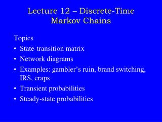
Lecture 12 – Discrete-Time Markov Chains. Topics State-transition matrix Network diagrams Examples: gambler’s ruin, brand switching, IRS, craps Transient probabilities Steady-state probabilities. Discrete – Time Markov Chains. Many real-world systems contain uncertainty and

E N D
Lecture 12 – Discrete-Time Markov Chains Topics • State-transition matrix • Network diagrams • Examples: gambler’s ruin, brand switching, IRS, craps • Transient probabilities • Steady-state probabilities
Discrete – Time Markov Chains Many real-world systems contain uncertainty and evolve over time. Stochastic processes (and Markov chains) are probability models for such systems. A discrete-time stochastic process is a sequence of random variables X0, X1, X2, . . . typically denoted by { Xn}. Origins: Galton-Watson process When and with what probability will a family name become extinct?
Components of Stochastic Processes The state space of a stochastic process is the set of all values that the Xn’s can take. (we will be concerned with stochastic processes with a finite # of states ) Time: n = 0, 1, 2, . . . State: v-dimensional vector, s = (s1, s2, . . . , sv) In general, there are m states, s1, s2, . . . , sm or s0, s1, . . . , sm-1 Also, Xn takes one of m values, so Xns.
If Xn = 4, then Xn+1 = Xn+2 = • • • = 4. If Xn = 0, then Xn+1 = Xn+2 = • • • = 0. Gambler’s Ruin At time 0 I have X0 = $2, and each day I make a $1 bet. I win with probability p and lose with probability 1– p. I’ll quit if I ever obtain $4 or if I lose all my money. State space is S = { 0, 1, 2, 3, 4 } Let Xn = amount of money I have after the bet on day n.
Markov Chain Definition A stochastic process { Xn} is called a Markov chain if Pr{Xn+1 = j | X0 = k0, . . . , Xn-1 = kn-1, Xn = i} = Pr{Xn+1 = j |Xn = i}transition probabilities for every i, j, k0, . . . , kn-1 and for every n. Discrete time means nN = {0, 1, 2, . . . }. The future behavior of the system depends only on the current state i and not on any of the previous states.
The one-step transition matrix for a Markov chain with states S = { 0, 1, 2 } is where pij = Pr{ X1 = j| X0 = i } Stationary Transition Probabilities Pr{Xn+1 = j |Xn = i } = Pr{ X1 = j |X0 = i } for all n (They don’t change over time) We will only consider stationary Markov chains.
Gambler’s Ruin Example 0 1 2 3 4 0 1 0 0 0 0 1 1-p 0 p 0 0 2 0 1-p 0 p 0 3 0 0 1-p 0 p 4 0 0 0 0 1 Properties of Transition Matrix If the state space S = {0, 1, . . . , m–1} then we have jpij= 1 i and pij 0 i, j (we must (each transition go somewhere) has probability 0)
Computer Repair Example • Two aging computers are used for word processing. • When both are working in morning, there is a 30% chance that one will fail by the evening and a 10% chance that both will fail. • If only one computer is working at the beginning of the day, there is a 20% chance that it will fail by the close of business. • If neither is working in the morning, the office sends all work to a typing service. • Computers that fail during the day are picked up the following morning, repaired, and then returned the next morning. • The system is observed after the repaired computers have been returned and before any new failures occur.
Index State State definitions 0 s = (0) No computers have failed. The office starts the day with both computers functioning properly. 1 s = (1) One computer has failed. The office starts the day with one working computer and the other in the shop until the next morning. 2 s = (2) Both computers have failed. All work must be sent out for the day. States for Computer Repair Example
Current state Events Prob-ability Next state 0 s0 = (0) Neither computer fails. 0.6 s' = (0) One computer fails. 0.3 s' = (1) Both computers fail. 0.1 s' = (2) 1 s1 = (1) Remaining computer does not fail and the other is returned. 0.8 s' = (0) Remaining computer fails and the other is returned. 0.2 s' = (1) 2 s2 = (2) Both computers are returned. 1.0 s' = (0) Events and Probabilities for Computer Repair Example Index
For computer repair example: State-Transition Matrix and Network The events associated with a Markov chain can be described by the mm matrix: P = (pij). For computer repair example, we have: • State-Transition Network • Node for each state • Arc from node i to node j if pij > 0.
Procedure for Setting Up a DTMC • Specify the times when the system is to be observed. • Define the state vector s = (s1, s2, . . . , sv) and list all the states. Number the states. • For each state s at time n identify all possible next states s' that may occur when the system is observed at time n + 1. • Determine the state-transition matrix P = (pij). • Draw the state-transition diagram.
Repair Operation Takes Two Days One repairman, two days to fix computer. new state definition required: s = (s1, s2) s1 = day of repair of the first machine s2 = status of the second machine (working or needing repair) For s1, assign 0 if 1st machine has not failed 1 if today is the first day of repair 2 if today is the second day of repair For s2, assign 0 if 2nd machine has not failed 1 if it has failed
State-Transition Matrix for 2-Day Repair Times 0 1 2 3 4 For example, p14 = 0.2 is probability of going from state 1 to state 4 in one day,where s1 = (1, 0) and s4 = (2, 1)
Brand Switching Example Number of consumers switching from brand i in week 26 to brand j in week 27 This is called a contingency table. Used to construct transition probabilities.
Empirical Transition Probabilities for Brand Switching, pij Steady state
Markov Analysis • State variable, Xn = brand purchased in week n • {Xn} represents a discrete state and discrete time stochastic process, where S= {1, 2, 3} and N = {0, 1, 2, . . .}. • If {Xn} has Markovian property and P is stationary, then a Markov chain should be a reasonable representation of aggregate consumer brand switching behavior. Potential Studies - Predict market shares at specific future points in time. - Assess rates of change in market shares over time. - Predict market share equilibriums (if they exist). - Evaluate the process for introducing new products.
Transform a Process to a Markov Chain Sometimes a non-Markovian stochastic process can be transformed into a Markov chain by expanding the state space. Example: Suppose that the chance of rain tomorrow depends on the weather conditions for the previous two days (yesterday and today). Specifically, Pr{ rain tomorrowrain last 2 days (RR) } = 0.7 Pr{ rain tomorrowrain today but not yesterday (NR) } = 0.5 Pr{ rain tomorrowrain yesterday but not today (RN) } = 0.4 Pr{ rain tomorrowno rain in last 2 days (NN) } = 0.2 Does the Markovian Property Hold?
The transition matrix: 0(RR) 1(NR)2(RN) 3(NN) 0 (RR) 0.7 0 0.3 0 P = 1 (NR)0.5 0 0.5 0 2 (RN) 0 0.4 0 0.6 3 (NN) 0 0.2 0 0.8 This is a discrete-time Markov process. The Weather Prediction Problem How to model this problem as a Markov Process ? The state space: 0 = (RR) 1 = (NR)2 = (RN) 3 = (NN)
Transition matrix Multi-step (n-step) Transitions The P matrix is for one step: n to n + 1. How do we calculate the probabilities for transitions involving more than one step? Consider an IRS auditing example: Two states: s0 = 0 (no audit), s1 = 1 (audit) Interpretation: p01 = 0.4, for example, is conditional probability of an audit next year given no audit this year.
The resultant matrix indicates, for example, that the probability of no audit 2 years from now given that the current year there was no audit is p00 = 0.56. (2) Two-step Transition Probabilities (2) Let pij be probability of going from i to j in two transitions. In matrix form, P(2) = P P, so for IRS example we have
The ij th entry of this reduces to pij(n) = pik(m) pkj(n-m) 1 mn1 m k=0 Chapman - Kolmogorov Equations n-Step Transition Probabilities This idea generalizes to an arbitrary number of steps. For n = 3: P(3) = P(2) P = P2 P = P3 or more generally, P(n) = P(m) P(n-m) Interpretation: RHS is the probability of going from i to k in m steps & then going from k to j in the remaining n m steps, summed over all possible intermediate states k.
n-Step Transition Matrix for IRS Example Time, n Transition matrix, P(n) 1 2 3 4 5
Gambler’s Ruin Revisited for p = 0.75 State-transition network State-transition matrix 0 1 2 3 4 0 1 0 0 0 0 1 0.25 0 0.75 0 0 2 0 0.25 0 0.75 0 3 0 0 0.25 0 0.75 4 0 0 0 0 1
Gambler’s Ruin with p = 0.75, n = 30 0 1 2 3 4 0 1 0 0 0 0 1 0.325 e0 e 0.675 2 0.1 0 e 0 0.9 3 0.025 e 0 e 0.975 4 0 0 0 0 1 P(30) = (eis very small nonunique number) What does matrix mean? A steady state probability does not exist.
Limiting probabilities 30-Step Transition Matrix for Gambler’s Ruin
Conditional vs. Unconditional Probabilities Let state space S = {1, 2, . . . , m}. Let pij be conditional n-step transition probability P(n). Let q(n) = (q1(n), . . . , qm(n)) be vector of all unconditional probabilities for all m states after n transitions. (n) Perform the following calculations: q(n) = q(0)P(n) or q(n) = q(n–1)P where q(0) is initial unconditional probability. The components of q(n) are called the transient probabilities.
Brand Switching Example We approximate qi(0) by dividing total customers using brand i in week 27 by total sample size of 500: q(0) = (125/500, 230/500, 145/500) = (0.25, 0.46, 0.29) To predict market shares for, say, week 29 (that is, 2 weeks into the future), we simply apply equation with n = 2: q(2) = q(0)P(2) = (0.327, 0.406, 0.267) = expected market share from brands 1, 2, 3
Transition Probabilities for n Steps Property 1: Let {Xn: n = 0, 1, . . .} be a Markov chain with state space Sand state-transition matrix P. Then for i and jS, and n = 1, 2, . . . Pr{Xn = j | X0 = i} = pij where the right-hand side represents the ijthelement of the matrix P(n). (n)
Brand switching example: π1 + π2 + π2 = 1, π1 0, π2 0, π3 0 Steady-State Probabilities Property 2: Let π = (π1, π2, . . . , πm) is the m-dimensional row vector of steady-state (unconditional) probabilities for the state space S = {1,…,m}. To find steady-state probabilities, solve linear system: π = πP, Sj=1,mπj = 1, πj 0, j = 1,…,m
Steady-State Equations for Brand Switching Example π1= 0.90π1 + 0.02π2 + 0.20π3 π2= 0.07π1 + 0.82π2 + 0.12π3 π3= 0.03π1 + 0.16π2 + 0.68π3 π1 + π2 + π3= 1 π1 0, π2 0, π3 0 Total of 4 equations in 3 unknowns Discard 3rd equation and solve the remaining system to get : π1= 0.474, π2= 0.321, π3= 0.205 Recall: q1(0) = 0.25, q2(0) = 0.46, q3(0) = 0.29
Comments on Steady-State Results • 1. Steady-state predictions are never achieved in actuality due to a combination of • (i) errors in estimating P • (ii) changes in P over time • (iii) changes in the nature of dependence relationships • among the states. • Nevertheless, the use of steady-state values is an important diagnostic tool for the decision maker. • Steady-state probabilities might not exist unless the Markov chain is ergodic.
For example, Existence of Steady-State Probabilities A Markov chain is ergodic if it is aperiodic and allows the attainment of any future state from any initial state after one or more transitions. If these conditions hold, then State-transition network 1 2 3 Conclusion: chain is ergodic. Craps
Game of Craps • The game of craps is played as follows. The player rolls a pair of dice and sums the numbers showing. • Total of 7 or 11 on the first rolls wins for the player • Total of 2, 3, 12 loses • Any other number is called the point. • The player rolls the dice again. • If she rolls the point number, she wins • If she rolls number 7, she loses • Any other number requires another roll • The game continues until he/she wins or loses
Game of Craps as a Markov Chain All the possible states Start Lose Win P4 P5 P6 P8 P9 P10 Continue
Game of Craps Network not (4,7) not (5,7) not (6,7) not (8,7) not (9,7) not (10,7) P6 P10 P5 P8 P4 P9 6 8 5 7 9 7 4 7 7 6 7 8 5 9 7 10 Win Lose 10 4 Start (7, 11) (2, 3, 12)
Game of Craps Probability of win = Pr{ 7 or 11 } = 0.167 + 0.056 = 0.223 Probability of loss = Pr{ 2, 3, 12 } = 0.028 + 0.056 + 0.028 = 0.112
q Roll, n ( n ) Start Win Lose P4 P5 P6 P8 P9 P10 q 0 (0) 1 0 0 0 0 0 0 0 0 q 1 (1) 0 0.222 0.111 0.083 0.111 0.139 0.139 0.111 0.083 q 2 (2) 0 0.299 0.222 0.063 0.08 0.096 0.096 0.080 0.063 q 3 (3) 0 0.354 0.302 0.047 0.058 0.067 0.067 0.058 0.047 q 4 (4) 0 0.394 0.359 0.035 0.042 0.047 0.047 0.042 0.035 q 5 (5) 0 0.422 0.400 0.026 0.030 0.032 0.032 0.030 0.026 Transient Probabilities for Craps This is not an ergodic Markov chain so where you start is important.
Interpretation of Steady-State Conditions • Just because an ergodic system has steady-state probabilities does not mean that the system “settles down” into any one state. 2. The limiting probability j is simply the likelihood of finding the system in state j after a large number of steps. 3. The probability that the process is in state j after a large number of steps is also equals the long-run proportion of time that the process will be in state j. 4. When the Markov chain is finite, irreducible and periodic, we still have the result that the πj, jS, uniquely solve the steady-state equations, but now πj must be interpreted as the long-run proportion of time that the chain is in state j.
What You Should Know About Markov Chains • How to define states of a discrete time process. • How to construct a state-transition matrix. • How to find the n-step state-transition probabilities (using the Excel add-in). • How to determine the unconditional probabilities after n steps • How to determine steady-state probabilities (using the Excel add-in).