Analyzing Differences II
Analyzing Differences II. Introduction to Communication Research School of Communication Studies James Madison University Dr. Michael Smilowitz. What to expect?. Describe the normal curve, Explain hypothesis testing. Null hypotheses Distinction between type I and type II errors.

Analyzing Differences II
E N D
Presentation Transcript
Analyzing Differences II Introduction to Communication Research School of Communication Studies James Madison University Dr. Michael Smilowitz
What to expect? • Describe the normal curve, • Explain hypothesis testing. • Null hypotheses • Distinction between type I and type II errors. • Discuss the logic behind tests of differences • Variance • Between group variance and within group variance
Galton’s Machine • Click on the following URL or copy it and paste it into your browser’s address bar. You will see a demonstration of Galton’s Machine. Note the “distribution” of where the balls land that occurs from “chance” alone. http://www.ms.uky.edu/~mai/java/stat/GaltonMachine.html
The Normal curve. 1 σ = 68.26% 1.96 σ = 95% 2.58 σ = 99%
The Normal curve. 1 σ = 68.26% 2.5 % 1.96 σ = 95% 2.5 % .5 % 2.58 σ = 99% .5 %
Hypothesis testing • A research hypothesis is an expectation about events based on generalizations of the assumed relationship between variables. • A null hypothesis states that there is no relationship between the variables. • Allows us to determine if the differences in sample means is the result of chance alone.
Hypothesis testing • If the null hypothesis is rejected, then the research hypothesis may be tenable and the researcher concludes that a relationship exists among variables. • If the null hypothesis is not rejected (logically you cannot “accept” a null hypothesis) then researchers can make no claim that a relationship exists among the variables.
Hypothesis testing Do you see why it is inappropriate to say “the hypothesis was proven”? All that is tested is the extent to which we can confidently say the observed relationships do not result from chance alone. So we can say: The hypothesis is not rejected. The results are valid indicators of a relationship. The findings support the hypothesis. • If the null hypothesis is rejected, then the research hypothesis may be tenable and the researcher concludes that a relationship exists among variables. • If the null hypothesis is not rejected (logically you cannot “accept” a null hypothesis) then researchers can make no claim that a relationship exists among the variables.
Definitions of Type I and Type II Errors: Smith (1988) A type I error, sometimes called an alpha error, results from rejecting a null hypothesis when it is true (p. 115). A type II error, sometimes called a beta error, results from failing to reject the null hypothesis when in fact it is false (p. 117)
Definitions of Type I and Type II Errors: Rinard (1994) Type I Error: Incorrectly rejecting the null hypothesis (p. 338). Type II Error: Failing to detect a relationship that is present; incorrectly failing to reject the null hypothesis (p. 338).
Analyzing Differences The question: Does the difference in the measurements of two (or more) samples represent “real” differences in the populations from which the samples are drawn? Researchers ask “Is the difference significant?”
Analyzing differences Tests of significant differences are based on the following ratio: The difference between the group (sample) means ________________________________________ An estimate of the error (chance) differences
Components of Variance The total variance (s2t) associated with any set of sample scores is comprised of (partitioned by)two components: The variation among scores due to some influence that “pushes” scores in one direction. Systematic Variance: The observed differences between groups is typically called the “between-group variance (s2b).
Components of Variance The total variance (s2t) associated with any set of sample scores is comprised of (partitioned by) two components: Fluctuations in group scores due to random or chance factors (errors such as fatigue, distractions, carelessness). Error Variance: Error variance is typically called the “within-group variance (s2w).
Components of Variance Therefore, the variance in a set of scores is: S2t = S2b + S2w
Got the point? Testing for the significance in the differences between samples is simply comparing the ratio of “between group variance” and “within group variance.”
Got the point? S2b ----------- S2w The greater the magnitude of S2b relative to S2w , the more confidently we expect the samples’ differences to indicate “real” differences in populations.