Software Performance Modeling
Software Performance Modeling. Dorina C. Petriu, Mohammad Alhaj, Rasha Tawhid Carleton University Department of Systems and Computer Engineering Ottawa, Canada, K1S 5B6 http://www.sce.carleton.ca/faculty/petriu.html. Analysis of Non-Functional Properties.

Software Performance Modeling
E N D
Presentation Transcript
Software Performance Modeling Dorina C. Petriu, Mohammad Alhaj, Rasha Tawhid Carleton University Department of Systems and Computer Engineering Ottawa, Canada, K1S 5B6 http://www.sce.carleton.ca/faculty/petriu.html
Analysis of Non-Functional Properties • Model-Driven Engineering enables the analysis of non-functional properties (NFP) of software models • examples of NFPs: performance, scalability, reliability, security, etc. • many existing formalisms and tools for NFP analysis • queueing networks, Petri nets, process algebras, Markov chains, fault trees, probabilistic time automata,formal logic, etc. • research challenge: bridge the gap between MDD and existing NFP analysis formalisms and tools rather than ‘reinventing the wheel’ • Approach: • add additional annotations for expressing different NFPs to software models • define model transformation from annotated software models to different NFP analysis models • using existing solvers, analyze the NFP models and give feedback to designers • In the UML world: define extensions as UML Profiles for expressing NFPs • UML Profile for Schedulability, Performance and Time (SPT) • UML Profile for Modeling and Analysis of Real-Time and Embedded systems (MARTE)
Software performance evaluation in MDE • Software performance evaluation in the context of Model-Driven Engineering: • starting point: UML software model used also for code generation • add performance annotations (using the MARTE profile) • generate a performance analysis model • queueing networks, Petri nets, stochastic process algebra, Markov chain, etc. • solve analysis model to obtain quantitative results • analyze results and give feedback to designers Model-to-code Transformation Software Code Code generation UML + MARTE Software Model UML Tool Model-to-model Transformation Performance Analysis Tool Performance Model Feedback to designers Performance Analysis Results Performance evaluation
PUMA transformation approach • PUMA project: Performance from Unified Model Analysis Software Core Transform model with Scenario Smodel to performance Model CSM annotations (CSM) (S2C) (Smodel) Transform Improve CSM to some Smodel Pmodel ( C 2 P ) Performance Performance Explore results and model solution design advice ( Pmodel ) space
Performance modeling formalisms • Analytic models • Queueing Networks (QN) • capture well contention for resources • efficient analytical solutions exists for a class of QN (“separable” QN): possible to derive steady-state performance measures without resorting to the underlying state space. • Stochastic Petri Nets • good flow models, but not as good for resource contention • Markov chain-based solution suffers from state space explosion • Stochastic Process Algebra • introduced in mid-90s by merging Process Algebra and Markov Chains • Stochastic Automata Networks • communicating automata synchronized by events; random execution times • Markov chain-based solution (corresponds to the system space state) • Simulation models • less constrained in their modeling power, can capture more details • harder to build and more expensive to solve (running the model repeatedly).
Queueing Networks (QN) • Queueing network model = a directed graph: • nodes are service centres, each representing a resource; • customers, representing the jobs, flow through the system and compete for these resources; • arcs with associated routing probabilities (or visit ratios) determine the paths that customers take through the network. • used to model systems with stochastic characteristics • multiple customer classes: each class has its own workload intensity (the arrival rate or number of customers), service demands and visit ratios • bottleneck service center: saturates first (highest demand, utilization) Open QN system Closed QN system
Queue length Residence Time Utilization Single Service Center: Non-linear Performance • Typical non-linear behaviour for queue length and waiting time • server reaches saturation at a certain arrival rate (utilization close to 1) • at low workload intensity: an arriving customer meets low competition, so its residence time is roughly equal to its service demand • as the workload intensity rises, congestion increases, and the residence time along with it • as the service center approaches saturation, small increases in arrival rate result in dramatic increases in residence time.
device entries task Layered Queueing Network (LQN) model http://www.sce.carleton.ca/rads/lqn/lqn-documentation • LQN is a extension of QN • models both software tasks (rectangles) and hardware devices (circles) • represents nested services (a server is also a client to other servers) • software components have entriescorresponding to different services • arcs represent service requests (synchronous, asynchronous and forwarding) • multi-servers used to model components with internal concurrency clientE ClientT Client CPU service1 service2 Appl Appl CPU query1 query2 DB DB CPU Disk1 Disk2
1..m 1..n Local Client Remote Client e1 e2 Local Wks RemoteWks Web Server e4 e3 Internet Web Proc a1 e5 & eComm Server a2 a3 & eComm Proc a4 [e4] Secure DB DB e7 e6 DB Proc Secure Proc Disk SDisk LQN extensions: activities, fork/join
package LQNmetamodel -fwdToEntry Processor Forward 1 -multiplicity : Integer = 1 -fwdByEntry -probForward -schedulerType 0..* -host 1 Call -callToEntry -allocatedTask 0..* 1 -meanCount ... Task 0..1 -multiplicity : Integer = 1 -callByActivity -priorityOnHost : Integer = 1 0..* -schedulerType -schedulableProcess 1 SyncCall -taskOperation 1..* -fwdTo Entry 1 0..1 -fwdBy AsyncCall 1 -callTo 1 -predecessor 1 -replyTo 0..* Precedence 1 -successor -firstActivity 1 1 0..1 1 Activity -actSetForEntry Sequence -thinkTime : float = 0.0 -hostDemand : float 0..* 1..* -after -hostDemCV : float = 1.0 Branch -deterministicFlag : Integer = 0 1..* -before -actSetForTask -repetitionsForLoop : float = 1.0 -probForBranch : float = 1.0 Merge 0..* -replyFwdFlag : Boolean Fork Phase1 Phase2 Join -replyFlag = true -replyFlag = False -successor.after = phase2 -successor = NIL ... LQN Metamodel
Performance versus Schedulability • Difference between performance and schedulability analysis • performance analysis: timing properties of best-effort and soft real-time systems • e.g., information processing systems, web-based applications and services, enterprise systems, multimedia, telecommunications • schedulability analysis: applied to hard real-time systems with strict deadlines • analysis often based on worst-case execution time, deterministic assumptions • Statistical performance results (analysis outputs): • mean (and variance) of throughput, delay (response time), queue length • resource utilization • probability of missing a target response time • Input parameters to the analysis - also probabilistic: • random arrival process • random execution time for an operation • probability of requesting a resource • Performance models represents a system at runtime • must include characteristics of software application and underlying platforms
General Resource Modeling Framework «profile» RTresourceModeling «import» «import» «profile» «profile» RTconcurrencyModeling RTtimeModeling «import» «import» «import» «profile» «modelLibrary» SAProfile RealTimeCORBAModel «import» «profile» RSAprofile UML SPT Profile Structure Analysis Models Infrastructure Models «profile» PAprofile
SPT Performance Profile: Fundamental concepts • Scenarios define execution paths with externally visible end points. • QoS requirements can be placed on scenarios. • Each scenario is executed by a workload: • open workload: requests arriving at in some predetermined pattern • closed workload: a fixed number of active or potential users or jobs • Scenario steps: the elements of scenarios joined by predecessor-successor relationships which may include forks, joins and loops. • a step may be an elementary operation or a whole sub-scenario • Resources are used by scenario steps. Quantitative resource demands for each step must be given in performance annotations. The main reason for building performance models is to compute additional delays due to the competition for resources! • Performance results include resource utilizations, waiting times, response times, throughputs. • Performance analysis is applied to real-time systems with stochastic characteristics and soft deadlines (use mean value analysis methods).
Resources Workload Scenario/ Step SPT Performance Profile: the domain model PerformanceContext 1 0..n 1 1..n 1..n 1..n PResource utilization schedulingPolicy throughput 1..n 1 0..n 0..n PScenario hostExecDemand responseTime Workload responseTime priority 0..n 1 {ordered} +root 1 1..n PStep probability repetition delay operations interval executionTime ClosedWorkload population externalDelay OpenWorkload occurencePattern +successor +host +predecessor 0..1 PPassiveResource waitingTime responseTime capacity accessTime PProcessingResource processingRate contextSwitchTime priorityRange isPreeemptible
MARTE domain model MarteFoundations MarteDesignModel MarteAnalysisModel MARTE overview • Foundations for modeling and analysis of RT/E systems : • CoreElements • NFPs • Time • Generic resource modeling • Generic component modeling • Allocation • Specialization of MARTE foundations for modeling purpose (specification, design, etc.): • RTE model of computation and communication • Software resource modeling • Hardware resource modeling Specialization of MARTE foundations for annotating models for analysis purpose: Generic quantitative analysis Schedulability analysis Performance analysis
GQAM dependencies and architecture • GQAM(Generic Quantitative Analysis Modeling):Common concepts for analysis • SAM:Modeling support for schedulability analysis techniques. • PAM:Modeling support for performance analysis techniques.
commRcvOvh and commTxOvh are host-specific costs of receiving and sending messages blockT describes a pure latency for the link «commHost» «commHost» internet: lan: {blockT = (100,us)} {blockT = (10,us), capacity = (100,Mb/s)} «execHost» «execHost» «execHost» webServerHost: dbHost: ebHost: {commRcvOverhead = (0.1,ms/KB), {commRcvOverhead = (0.14,ms/KB), {commRcvOverhead = (0.15,ms/KB), commTxOverhead = (0.2,ms/KB)} commTxOverhead = (0.07,ms/KB), commTxOverhead = (0.1,ms/KB), resMult = 3} resMult = 5} «deploy» «deploy» «deploy» «artifact» «artifact» «artifact» webServerA databaseA ebA «manifest» resMult = 5 describes a symmetric multiprocessor with 5 processors «manifest» «manifest» : EBrowser : WebServer : Database Annotated deployment diagram
Simple scenario a swimlane or lifeline stereotyped «PaRunTInstance» references a runtime active instance; poolSize specifies the multiplicity initial step is stereotypedfor workload (open), execution demand request message size «PaRunTInstance» «PaRunTInstance» «PaRunTInstance» webServer: WebServer database: Database eb: EBrowser {poolSize = (webthreads=80), {poolSize = (dbthreads=5), instance = webserver} instance = database} 1: 2: «PaWorkloadEvent» «paStep» {open (interArrT=(exp(17,ms))), «paCommStep» «PaStep» {hostDemand = (4.5,ms)} {hostDemand = (12.4,ms), «paCommStep» rep = (1.3,-,mean), msgSize = (2,KB)} 3: «paCommStep» 4: {msgSize = (50,KB)} «PaCommStep» {msgSize = (75,KB)}
UML model for performance analysis • For performance analysis, a UML model should contain: • Key use cases realized by representative scenarios • frequently executed, with performance constraints • each scenario is a graph of steps (partial ordering) • Resources used by each scenario • resource types: active or passive, physical or logical, hardware or software • examples: processor, disk, process, software server, lock, buffer • quantitative resource demands for each scenario step • how much, how many times? • Workload intensity for each scenario • open workload: arrival rate of requests for the scenario • closed workload: number of simultaneous users
Direct UML to LQN Transformation: our first approach • Mapping principle: • software and hardware resources → service centres • scenarios → job flow from centre to centre • Generate LQN model structure (tasks, devices and their connections) from the structural view: • active software instances → LQN tasks • map deployment nodes → LQN devices • Generate LQN detailed elements (entries, phases, activities and their parameters) from the behavioural view: • identify communication patterns in key scenarios due to architectural patterns • client/server, forwarding server chain, pipeline, blackboard, etc. • aggregate scenario steps according to each pattern and map to entries, phases, etc. • compute LQN parameters from resource demands of scenario steps.
Client Client Server Server CLIENT SERVER CLIENT SERVER Client Server Client Server 1..n <<process>> <<process>> <<process>> <<process>> <<process>> Client Server Server Database Database <<disk>> Generating the LQN model structure a) High-level architecture Generated LQN model structure Client Client Client Client Server Server Server Server CLIENT SERVER CLIENT SERVER CLIENT SERVER CLIENT SERVER Client Modem Client Client Server Server Client Client Server Server ProcC 1..n 1..n <<process>> <<process>> <<process>> <<process>> <<process>> <<process>> Client User WebServer Server Database Database Internet WebServer ProcS b) Deployment LAN Database ProcC1 ProcC1 ProcCN ProcCN ProcDB User1 Client1 ClientN UserN <<Modem>> <<Modem>> <<Modem>> <<Modem>> Disk1 <<Internet>> <<Internet>> • Software tasks generated for high-level software components according to the architectural patterns used. • Hardware tasks generated for devices from deployment diagram <<LAN>> <<LAN>> ProcS ProcS ProcDB ProcDB WebServer Server Database Database <<disk>> Disk1
Client Server Pattern • Structure • the participants and their relationship • Behaviour • Synchronous communication style - the client sends the request and remains blocked until the sender replies Client Server Client Sever ClientServer request service waiting 1..n 1 Client Server serve request and reply wait for reply complete service (opt) continue work a) Client Sever collaboration b) Client Sever behaviour
e1 [ph1] e1, ph1 e2, ph1 e2 [ph1, ph2] e2, ph2 Mapping the Client Server Pattern to LQN Client Client User User WebServer WebServer Server Server LQN waiting waiting request request request request service service service service Client serve request wait for reply and reply and reply Client CPU e1, ph1 ... Server complete complete continue continue work work service (opt) Server CPU For each subset of scenario steps mapped to a LQN phase or activity, compute the execution time S: S = Si=1,n ri si where ri = number of repetitions and si = execution time of step i.
e1 [ph1] Identify patterns in a scenario UserInterface ECommServ DBMS LQN browse and select items idle <<PAstep>> {PArep= $r} User Interface <<PAstep>> {PAdemand= ‘assm’, ’mean’, $md1, ‘ms’} phase 1 check valid item code <<PAstep>> {PAdemand= ‘assm’, ’mean’, $md2, ‘ms’} add item to query EComm Server <<PAstep>> {PAdemand= ‘assm’, ’mean’, $md3, ‘ms’} e2 [ph1] waiting phase 1 sanitize query idle e3 DBMS phase 1 [ph1, ph2] waiting add to invoice generate page phase 2 display <<PAstep>> {PAdemand= ‘assm’, ’mean’, $md3, ‘ms’} log transaction
Pivot language, also called a bridge or intermediate language, can be used as an intermediary for translation. Avoids the combinatorial explosion of translators across every combination of languages. Examples of pivot languages for performance analysis: Core Scenario Model (CSM) Klaper PMIF + S-PMIF Palladio Model Transformations from N source languages to M target languages require N*M transformations. L’1 L1 L’2 L2 . . . . . . L’M LN L1 L’1 Lp L’2 L2 . . . . . . L’M LN Pivot languages • Using a pivot language, only N+M transformations. Also, a smaller semantic gap
UML+SPT LQN CSM UML+MARTE QN UCM Petri Net Simulation Core Scenario Model • CSM: a pivot Domain Specific Language used in the PUMA project at Carleton University (Performance from Unified Model Analysis) • Semantically – between the software and performance domains • focused on scenarios and resources • performance data is intrinsic to CSM • quantitative resource demands made by scenario steps • workload PUMA Transformation chain
Scenario/steps Resources Workload CSM Metamodel
CSM metamodel • Basic scenario elements, similar to the SPT Performance Profile • scenario composed of steps • a step may be refined as a sub-scenario • precedence relationships among steps • sequence, branch, merge, fork, join, loop • steps performed by components running on hosts (Processor resources) • resources and acquire/release operations on resources • inferred for Component-based resources (Processes) • Four kinds of resources in CSM: • ProcessingResource (a node in a deployment diagram) • ComponentResource (process, or active object) • component in a deployment • lifeline in SD may correspond to a runtime component • swimlane in AD may correspond to a runtime component • LogicalResource (declared as GRMresource) • extOp resource - implied resource to execute external operations
CORBA-based case study • Two CORBA-based client-server systems: • H-ORB (handle-driven ORB): the client gets the address of the server from the agent and communicates with the server directly. • F-ORB (forwarding ORB): the agent forwards the client request to the appropriate server, which returns the results of the computations directly to the client. • Synthetic application: • Contains two services A and B; two copies of each service are provided; • The clients connect to these services through the ORB. • Each client executes a cycle repeatedly, making one request to Server A (distributed randomly between copies A1 and A2) and one to Server B (distributed randomly between copies B1 and B2). • The client performs a bind operation before every request. • Since the experiments were performed on a local area network, the inter-node delay that would appear in a wide-area network was simulated by making a sender process sleep for D units of time before sending a message.
H-ORB deployment and scenario Deployment Scenario as activity diagram
«GaAnalysisContext» sd HORB «PaRunTInstance» «PaRunTInstance» «PaRunTInstance» «PaRunTInstance» «PaRunTInstance» «PaRunTInstance» Client Agent ServerA1 ServerA2 ServerB1 ServerB2 «GaWorkloadEvent» ref Sleep {pattern=(closed(Population= $N))} GetHandle() «PaStep» {hostDemand=(4,ms)} ref Sleep ref Sleep alt «PaStep» «PaStep» {hostDemand=($SA,ms)} {prob=0.5} A1Work() ref Sleep «PaStep» «PaStep» {hostDemand=($SA,ms)} {prob=0.5} A2Work() ref Sleep ref Sleep GetHandle() «PaStep» {hostDemand=(4,ms)} ref Sleep ref Sleep «PaStep» {prob=0.5} alt «PaStep» {hostDemand=($SB,ms)} B1Work() ref Sleep «PaStep» {prob=0.5} «PaStep» {hostDemand=($SB,ms)} B2Work() ref Sleep H-ORB scenario as sequence diagram
Structural elements are generated first: CSM ProcessingResource CSM Component Scenarios described by SD CSM Start PathConnection is generated first, and the workload information is attached to it Lifelines stereotyped «PaRunTInstance» correspond to an active runtime instance The translation follows the message flow of the scenario, generating corresponding Steps and PathConnections a UML Execution Occurrence generates a simple Step Complex CSM Steps with a nested scenario correspond to operand regions of UML Combined Fragments and Interaction Occurrences. Transformation from UML+MARTE to CSM Mapping of MARTE stereotypes to CSM model elements
«GaAnalysisContext» sd HORB «PaRunTInstance» «PaRunTInstance» «PaRunTInstance» «PaRunTInstance» «PaRunTInstance» «PaRunTInstance» Client Agent ServerA1 ServerA2 ServerB1 ServerB2 «GaWorkloadEvent» ref Sleep {pattern=(closed(Population= $N))} GetHandle() «PaStep» {hostDemand=(4,ms)} ref Sleep ref Sleep alt «PaStep» «PaStep» {hostDemand=($SA,ms)} {prob=0.5} A1Work() ref Sleep «PaStep» «PaStep» {hostDemand=($SA,ms)} {prob=0.5} A2Work() ref Sleep ref Sleep GetHandle() «PaStep» {hostDemand=(4,ms)} ref Sleep ref Sleep «PaStep» {prob=0.5} alt «PaStep» {hostDemand=($SB,ms)} B1Work() ref Sleep «PaStep» {prob=0.5} «PaStep» {hostDemand=($SB,ms)} B2Work() ref Sleep Transformation from SD to CSM
Transformation from CSM to LQN • The first transformation phase parses the CSM resources and generates: • a LQNTask for each CSM Component • a LQN Processorfor each CSM ProcessingResource • The second transformation phase traverses the CSM to determine: • the branching structure and the sequencing of Steps within branches • the calling interactions between Components. • A new LQN Entry is generated whenever a task receives a call • The entry internals are described by LQNActivities that represent a graph of CSM Steps or by Phases. LQN model for the H-ORB system
Validation of LQN against measurements • The LQN results are compared with measurements of the implementation of a performance prototype based on a Commercial-Off-The-Shelf (COTS) middleware product and a synthetic workload running on a network of Sun workstations using Solaris 2.6 H-ORB F-ORB
Extensions Smodel adapted to service-based systems: Business process model Service model Separation between: PIM: platform independent PSM: platform specific Use Performance Completion feature model to specify platform variability Techniques Use Aspect-oriented Models for platform operations aspect composition may take place at different levels: UML, CSM, LQN Traceability between different kinds of models PUMA4SOA approach
Eligibility Referral System (ERS) Source PIM: (a) Business Process Model
Source PIM: (b) Service Architecture Model <<Participant>> • SoaML stereotypes: • <<Participant>>indicates parties that provides or consumes services. • <<Request>> indicates the consumption of a service. • <<Service>> indicates the offered service. <<Participant>> as:AdmissionServer <<Participant>> na:NursingAccount es:EstimatorServer <<Service>> <<Request>> <<Request>> <<Service>> validateTransfer validateTransfer payorAuth payorAuth <<Service>> <<Request>> <<Request>> confirmTransfer <<Participant>> confirmTransfer recordTransfer dm:Datamanagement <<Request>> <<Service>> <<Request>> <<Participant>> physicianAuth pa:PhysicianAccount recordTransfer scheduleTransfer <<Service>> <<Request>> scheduleTransfer <<Service>> requestReferral physicianAuth <<Service>> requestReferral
join points for platform aspects Source PIM: (c) Service Behaviour Model
Models describing the platform Admission node Insurance node Transferring node Deployment of the primary model
Service Platform Data Compression Message Protocol Realization Communication <1 - 1> <1 - 1> <1 - 1> << Feature >> << Feature >> <1 - 1> <<Feature >> <<Feature >> <<Feature >> <<Feature >> DCOM Web service Compressed Uncompressed Http SOAP << Feature >> << Feature >> << Feature >> << Feature >> Unsecure R EST Secure CORBA <1 - 1> Operation << Feature >> << Feature >> << Fea ture >> SSL Protocol TSL Protocol << Feature >> <1 - 1> Invocation Discovery << Feature >> << Feature >> Subscribing Publishing Performance Completion Feature Model • Describes the variability in the service platform • The Service Platform feature model in the example defines: • three mandatory feature groups: Operation, Message Protocol and Realization • two optional feature groups: Communication and Data compression • Each feature is described by an aspect model to be composed with the base model
Generic Aspect Model: e.g. Service Invocation Aspect defines the structure and behavior of the platform aspect in a generic format uses generic names (i.e., formal parameters) for software and hardware resources uses generic performance annotations (MARTE variables) Advantage: reusability Context-specific aspect model: after identifying a join point, the generic aspect model is bound to the context of the join point the context-specific aspect model is composed with the platform model Generic Aspect Model: Service Invocation
Binding generic to concrete resources • Generic names (parameters) are bound to concrete names corresponding to the context of the join point • Sometime new resources are added to the primary model • User input is required (e.g., in form of Excel spreadsheet, as discussed later).
Binding performance annotation variables • Annotation variables allowed in MARTE are used as generic performance annotations • Bound to concrete reusable platform-specific annotations
composed service invocation aspect composed service response aspect PSM: scenario after composition in UML