Download
1 / 48
480 likes | 606 Vues
This document covers essential topics in statistical inference concerning quantitative variables, focusing on the t-distribution and its applications. It addresses single means, differences in means, matched pairs, and correlation, underscoring the importance of normality assumptions and degrees of freedom. Included are homework assignments and project deadlines related to these concepts, as well as practical applications such as hypothesis testing using a real-world example involving Chips Ahoy! cookies.

E N D
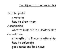
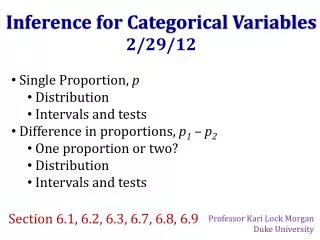
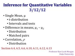
Inference for Quantitative Variables • 3/12/12 • Single Mean, µ • t-distribution • Intervals and tests • Difference in means, µ1 – µ2 • Distribution • Matched pairs • Correlation, • Distribution • Section 6.4, 6.5, 6.6, 6.10, 6.11, 6.12, 6.13 • Professor Kari Lock Morgan • Duke University
To Do • Homework 6 (due Monday, 3/19) • Project 1 (due Thursday, 3/22)
Inference Using N(0,1) If the distribution of the sample statistic is normal: A confidence interval can be calculated by where z*is a N(0,1) percentile depending on the level of confidence. A p-value is the area in the tail(s) of a N(0,1) beyond
CLT for a Mean Population Distribution of Sample Data Distribution of Sample Means n = 10 n = 30 n = 50
SE of a Mean • The standard error for a sample mean can be calculated by
Standard Deviation • The standard deviation of the population is • • s
Standard Deviation • The standard deviation of the sample is • • s
Standard Deviation • The standard deviation of the sample mean is • • s
CLT for a Mean • If n ≥ 30*, then *Smaller sample sizes may be sufficient for symmetric distributions, and 30 may not be sufficient for very skewed distributions or distributions with high outliers
Standard Error • We don’t know the population standard deviation , so estimate it with the sample standard deviation, s
t-distribution • Replacing with s changes the distribution of the z-statistic from normal to t • The t distribution is very similar to the standard normal, but with slightly fatter tails to reflect this added uncertainty
Degrees of Freedom • The t-distribution is characterized by itsdegrees of freedom (df) • Degrees of freedom are calculated based on the sample size • The higher the degrees of freedom, the closer the t-distribution is to the standard normal
t-distribution To calculate area in the tail(s), or to find percentiles of a t-distribution, use http://surfstat.anu.edu.au/surfstat-home/tables/t.php
Normality Assumption • Using the t-distribution requires an extra assumption: the data comes from a normal distribution • Note: this assumption is about the original data, not the distribution of the statistic • For large sample sizes we do not need to worry about this, because s will be a very good estimate of , and t will be very close to N(0,1) • For small sample sizes (n < 30), we can only use the t-distribution if the distribution of the data is approximately normal
Normality Assumption • One small problem: for small sample sizes, it is very hard to tell if the data actually comes from a normal distribution! Population Sample Data, n = 10
Small Samples • If sample sizes are small, only use the t-distribution if the data looks reasonably symmetric and does not have any extreme outliers. • Even then, remember that it is just an approximation! • In practice/life, if sample sizes are small, you should just use simulation methods (bootstrapping and randomization)
Confidence Intervals df = n – 1 t* is found as the appropriate percentile on a t-distribution with n – 1 degrees of freedom IF n is large or the data is normal
Hypothesis Testing df = n – 1 The p-value is the area in the tail(s) beyond t in a t-distribution with n – 1 degrees of freedom, IF n is large or the data is normal
Chips Ahoy! ? A group of Air Force cadets bought bags of Chips Ahoy! cookies from all over the country to verify this claim. They hand counted the number of chips in 42 bags. Source: Warner, B. & Rutledge, J. (1999). “Checking the Chips Ahoy! Guarantee,” Chance, 12(1).
Chips Ahoy! Can we use hypothesis testing to prove that there are 1000 chips in every bag? (“prove” = find statistically significant) (a) Yes (b) No
Chips Ahoy! Can we use hypothesis testing to prove that the average number of chips per bag is 1000? (“prove” = find statistically significant) (a) Yes (b) No
Chips Ahoy! Can we use hypothesis testing to prove that the average number of chips per bag is more than 1000? (“prove” = find statistically significant) (a) Yes (b) No
Chips Ahoy! ? • Are there more than 1000 chips in each bag, on average? • (a) Yes • (b) No • (c) Cannot tell from this data • Give a 99% confidence interval for the average number of chips in each bag.
Chips Ahoy! 1. State hypotheses: 2. Check conditions: 3. Calculate test statistic: 4. Compute p-value: > pt(14.4, df=41, lower.tail=FALSE) [1] 6.193956e-18 4. Interpret in context: This provides extremely strong evidence that the average number of chips per bag of Chips Ahoy! cookies is significantly greater than 1000.
Chips Ahoy! 1. Check conditions: 2. Find t*: 4. Compute confidence interval: 4. Interpret in context: We are 99% confident that the average number of chips per bag of Chips Ahoy! cookies is between 1212.6 and 1310.6 chips.
t-distribution Which of the following properties is/are necessary for to have a t-distribution? the data is normal the sample size is large the null hypothesis is true a or b d and c
SE for Difference in Means df = smaller of n1 – 1 and n2 – 1
CLT for Difference in Means *Smaller sample sizes may be sufficient for symmetric distributions, and 30 may not be sufficient for skewed distributions
t-distribution • For a difference in means, the degrees of freedom for the t-distribution is the smaller of n1 – 1 and n2 – 1 • The test for a difference in means using a t-distribution is commonly called a t-test
The Pygmalion Effect Teachers were told that certain children (chosen randomly) were expected to be “growth spurters,” based on the Harvard Test of Inflected Acquisition (a test that didn’t actually exist). These children were selected randomly. The response variable is change in IQ over the course of one year. • Source: Rosenthal, R. and Jacobsen, L. (1968). “Pygmalion in the Classroom: Teacher Expectation and Pupils’ Intellectual Development.” Holt, Rinehart and Winston, Inc.
The Pygmalion Effect Does this provide evidence that merely expecting a child to do well actually causes the child to do better? (a) Yes (b) No If so, how much better? *s1 and s2 were not given, so I set them to give the correct p-value
Pygmalion Effect 1. State hypotheses: 2. Check conditions: 3. Calculate t statistic: 4. Compute p-value: 5. Interpret in context: We have evidence that positive teacher expectations significantly increase IQ scores in elementary school children.
Pygmalion Effect From the paper: “The difference in gains could be ascribed to chance about 2 in 100 times”
Pygmalion Effect 1. Check conditions: 2. Find t*: 3. Compute the confidence interval: 4. Interpret in context: We are 95% confident that telling teachers a student will be an intellectual “growth spurter” increases IQ scores by between 0.17 and 7.43 points on average, after 1 year.
Matched Pairs • A matched pairs experiment compares units to themselves or another similar unit, rather than just compare group averages • Data is paired(two measurements on one unit, twin studies, etc.). • Look at the difference in responses for each pair
Pheromones in Tears • Do pheromones (subconscious chemical signals) in female tears affect testosterone levels in men? • Cotton pads had either real female tears or a salt solution that had been dripped down the same female’s face • 50 men had a pad attached to their upper lip twice, once with tears and once without, order randomized. • Response variable: testosterone level Gelstein, et. al. (2011) “Human Tears Contain a Chemosignal," Science, 1/6/11.
Matched Pairs Why do a matched pairs experiment? Decrease the standard deviation of the response Increase the power of the test Decrease the margin of error for intervals All of the above None of the above
Matched Pairs • Matched pairs experiments are particularly useful when responses vary a lot from unit to unit • We can decrease standard deviation of the response (and so decrease standard error of the statistic) by comparing each unit to a matched unit
Matched Pairs • For a matched pairs experiment, we look at the difference between responses for each unit, rather than just the average difference between treatment groups • Get a new variable of the differences, and do inference for the difference as you would for a single mean
Pheromones in Tears • The average difference in testosterone levels between tears and no tears was -21.7 pg/ml. • The standard deviation of these differences was 46.5 • Average level before sniffing was 155 pg/ml. • The sample size was 50 men • Do female tears lower male testosterone levels? • (a) Yes (b) No (c) ??? • By how much? Give a 95% confidence interval. “pg” = picogram = 0.001 nanogram = 10-12 gram
Pheromones in Tears 1. State hypotheses: 2. Check conditions: 3. Calculate test statistic: 4. Compute p-value: > pt(-3.3, df=49, lower.tail=TRUE) [1] 0.000903654 5. Interpret in context: This provides strong evidence that female tears decrease testosterone levels in men, on average.
Pheromones in Tears 1. Check conditions: 2. Find t*: > qt(0.975 df=49) [1] 2.009575 3. Compute the confidence interval: 4. Interpret in context: We are 95% confident that female tears on a cotton pad on a man’s upper lip decrease testosterone levels between 8.54 and 34.86 pg/ml, on average.
Correlation t-distribution df = n - 2
Social Networks and the Brain • Is the size of certain regions of your brain correlated with the size of your social network? • Social network size measured by many different variables, one of which was number of facebook friends. Brain size measured by MRI. • The sample correlation between number of Facebook friends and grey matter density of a certain region of the brain (left middle temporal gyrus), based on 125 people, is r = 0.354. Is this significant? (a) Yes (b) No Source: R. Kanai, B. Bahrami, R. Roylance and G. Ree (2011). “Online social network size is reflected in human brain structure,” Proceedings of the Royal Society B: Biological Sciences. 10/19/11.
Social Networks and the Brain 1. State hypotheses: 2. Check conditions: 3. Calculate test statistic: 4. Compute p-value: > pt(4.2, df=123,lower.tail=FALSE) [1] 2.539729e-05 5. Interpret in context: This provides strong evidence that the size of the left middle temporal gyrus and number of facebook friends are positively correlated.