Sorting

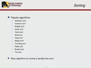
1. Sorting • Popular algorithms: • Selection sort * • Insertion sort* • Bubble sort* • Quick sort* • Comb-sort • Shell-sort • Heap sort* • Merge sort* • Counting-sort • Radix-sort • Bucket-sort • Tim-sort • Many algorithms for sorting in parallel also exist.

2. Selection Sort • Sorting Algorithm #1: Selection sort • Very easy to understand and implement. • Not very efficient.

3. Selection Sort // Selection sort in Java publicstaticvoid sort(int[] a){ int minPos, temp; for (int i=0; i<=a.length-2; i++){ // Find the position of the value that belongs in position i minPos = i; for (int j=i+1; j<=a.length-1; j++) if (a[j] < a[minPos]) minPos = j; // Swap the values in positions i and min temp = a[i]; a[i] = a[minPos]; a[minPos] = temp; } } Running time? Θ(n2) – best, worst, average

4. Selection Sort

5. Insertion Sort • Sorting Algorithm #2: Insertion sort • Also very easy to understand and implement. • Also not very efficient.

6. // Insertion sort publicstaticvoid insertionSort(int[] a) { int j; for (int i=1; i<=a.length-1; i++) { j=i; while (j>=1) { if (a[j] < a[j-1]) { temp=a[j-1]; a[j-1]=a[j]; a[j]=temp; } j=j-1; } } } Insertion Sort • Initial version: Running time? Θ(n2) – best, worst, average Analysis is same as for Selection-sort

7. // This one eliminates the boolean variable public static void insertionSort(int[] a) { int j; for (int i=1; i<=a.length-1; i++) { j=i; while ((j>=1) && (a[j]<a[j-1])) { temp=a[j-1]; a[j-1]=a[j]; a[j]=temp; j = j – 1; } } } Insertion Sort • Second version: Running time? Θ(n2) – worst (list in reverse order) Θ(n) – best (list already sorted)

8. Insertion Sort • More Technically, assuming the list is already sorted… • On the ith iteration of the outer loop, as i goes from 1 to a.length-1, the inner loop executes exactly 1 time. • This gives a total of n iterations of the inner loop. • Again, note that we only counted the number of iterations of the inner loop.

9. Insertion Sort // Another slight improvement in efficiency public static void insertionSort(int[] a) { int j, v; for (int i=1; i<=a.length-1; i++) { j=i; v = a[j]; while ((j>=1) && (v<a[j-1])) { a[j]=a[j-1]; j=j-1; } a[j] = v; } } • Third version: Running time? Θ(n2) – worst (list in reverse order) Θ(n) – best (list already sorted)

10. Bubble Sort • Sorting Algorithm #3: Bubble sort • Also very easy to understand and implement. • Also not very efficient. • Several minor variations and enhancements are possible.

11. // Bubble sort public static void bubbleSort1(int[] a) { int temp; for (int i=1; i<=a.length-1; i++) { for (int j=0; j<a.length-i; j++) { if (a[j] > a[j+1]) { temp = a[j]; a[j] = a[j+1]; a[j+1] = temp; } } } } Bubble Sort • Initial version: Running time? Θ(n2) – best, worst, average Analysis is same as for Selection-sort

12. // This version stops when a pass occurs with no swaps. public static void bubbleSort1(int[] a) { int i, temp; boolean doMore; i = 1; doMore = true; while ((i<=a.length-1) && (doMore)) { doMore = false; for (int j=0; j<a.length-i; j++) if (a[j] > a[j+1]) { temp = a[j]; a[j] = a[j+1]; a[j+1] = temp; doMore = true; } i = i + 1; } } Bubble Sort • Second version: (fewer bubbles) Running time? Θ(n2) – worst (list in reverse order) Θ(n) – best (list already sorted)

13. Bubble Sort • More Technically, assuming the list is already sorted… • On the 1st iteration of the outer loop, inner loop executes exactly n times. • The outer loops only executes 1. • Again, note that we only counted the number of iterations of the inner loop.

14. Quick Sort • Sorting Algorithm #4: Quick sort • Proposed by C.A.R. Hoare in1962. • Divide-and-conqueralgorithm. • More efficient than selection, insertion, or bubble sort, on average. • Worst case is just as bad -Θ(n2) • Very practical.

15. Quick Sort • Divide: Partition the array into two subarrays around a pivot x such that elements in lower subarray x  elements in upper subarray. • Conquer: Recursively sort the two subarrays. • Combine: Trivial. Key: Linear-time partitioning subroutine. x x x ≤x ≥x x

16. Quick Sort • Partitioning algorithm from the book: PARTITION(A,p,q) A[ p . .q] x A[p] pivot = A[p] i p for j p + 1 toq do if A[ j] x then i i + 1 exchange A[i] A[ j] exchange A[ p] A[i] return i

17. Quick Sort i j

18. Quick Sort i j

19. Quick Sort j i

20. Quick Sort i j

21. Quick Sort j i

22. Quick Sort j i

23. Quick Sort i j

24. Quick Sort j i

25. Quick Sort i j

26. Quick Sort j i

27. Quick Sort j i

28. Quick Sort i

29. QUICKSORT(A, p, r) if p < r then q PARTITION(A, p, r) QUICKSORT(A, p, q–1) QUICKSORT(A, q+1, r) Initial call: QUICKSORT(A, 1, n)

30. Quick Sort

31. Quick Sort • What would partition do in the worst-case? i j

32. Quick Sort – Recursion Tree T(n) = T(0) + T(n–1) +cn T(n)

33. Worst Case Recursion Tree T(n) = T(0) + T(n–1) +cn cn T(0) T(n–1)

34. Quick Sort – Recursion Tree T(n) = T(0) + T(n–1) +cn cn T(0) c(n–1) T(0) T(n–2)

35. Quick Sort – Recursion Tree T(n) = T(0) + T(n–1) +cn cn T(0) c(n–1) T(0) c(n–2) T(0) … (1)

36. Quick Sort – Recursion Tree T(n) = T(0) + T(n–1) +cn cn T(0) c(n–1) T(0) c(n–2) T(0) … (1)

37. Quick Sort – Recursion Tree T(n) = T(0) + T(n–1) +cn cn (1) c(n–1) T(n) = (n) +(n2) =(n2) (1) c(n–2) h =n (1) … (1)

38. Quick Sort • Best case analysis: If we get lucky, partition splits the array evenly T(n) = 2T(n/2) + Θ(n) = Θ(nlgn) (same as Merge-Sort) • What if the split is 1/10 : 9/10? T(n) = T(n/10) + T(n/10) + Θ(n) = Θ(nlgn) (left as an exercise – recursion tree) • In fact, any split by a constant proportional amount will lead to Θ(nlgn)

39. Quick Sort • What if alternates between best and worst cases: L(n) = 2U(n/2) + Θ(n) U(n) = L(n-1) + Θ(n) • Solution: L(n) = 2U(n/2) + Θ(n) = (2L(n/2 - 1) + Θ(n/2)) + Θ(n) = 2L(n/2 - 1) + Θ(n) = Θ(nlgn) (left as an exercise)

40. Heap Sort • In this context, the term heap has nothing to do with memory organization! • Heap properties: • Forms an almost-complete binary tree, i.e., completely filled on all levels, except possibly the lowest, which is filled from the left up to some point. • The value at any given node is greater than the value of both it’s children (max-heap). • The root will have the largest value. 16 14 10 8 7 9 3 2 4 1

41. Heap Sort • An important operation on heaps is Max-Heapify, which pushes a value down the tree if it violates the heap property. 5 14 10 8 7 9 3 2 4 1

42. Heap Sort • In such a case, Max-Heapify will swap the value with the larger of it’s two children and then repeat. 5 14 10 8 7 9 3 2 4 1

43. Heap Sort • In such a case, Max-Heapify will swap the value with the larger of it’s two children and then repeat. 14 5 10 8 7 9 3 2 4 1

44. Heap Sort • In such a case, Max-Heapify will swap the value with the larger of it’s two children and then repeat. 14 8 10 7 9 3 5 2 4 1

45. Heap Sort • Sometimes Max-Heapify will push a value all the way to the leaf-level. 3 14 10 8 7 9 3 2 4 1

46. Heap Sort • Sometimes Max-Heapify will push a value all the way to the leaf-level. 14 3 10 8 7 9 3 2 4 1

47. Heap Sort • Sometimes Max-Heapify will push a value all the way to the leaf-level. 14 8 10 7 9 3 3 2 4 1

48. Heap Sort • Sometimes Max-Heapify will push a value all the way to the leaf-level. 14 8 10 4 7 9 3 3 2 1

49. Heap Sort 16 14 10 For the above: A.length= 12 A.heap-size = 10 8 7 9 3 2 4 1

50. Heap Sort • The Max-Heapify procedure can then be specified as: