Download
1 / 15
150 likes | 284 Vues
CO and CO 2 Diurnal Cycles during CalNex -LA, 15 May - 16 June, 2010. Sally Newman 1 , Sergio Alvarez 2 , Bernhard Rappenglueck 2 , Charles E. Miller 3 , and Yuk L. Yung 1

E N D
CO and CO2 Diurnal Cycles during CalNex-LA, 15 May - 16 June, 2010 Sally Newman1, Sergio Alvarez2, Bernhard Rappenglueck2, Charles E. Miller3, and Yuk L. Yung1 1Geological and Planetary Sciences, Caltech, Pasadena, CA; 2Atmospheric and Earth Sciences, Univ. Houston, Houston, TX; 3Earth Atmospheric Sciences, JPL, Pasadena, CA
c. Trailer city of the CalNex site. Photo by Michael Lechner. a. Location of Pasadena. Figure 1. b. Location of the CalNex-LA site on the Caltech campus.
Introduction SInce more than half of the world’s population lives in urban regions, which contribute a disproportionate amount of greenhouse gases and other pollutants to the atmosphere, it is important to understand cycles in the sources of these components in cities. We investigated the relationships between the diurnal cycles of CO2 and CO using high precision atmospheric concentration measurements collected during the CalNex-LA ground campaign of 15 May - 15 June, 2010. The location of this campaign is shown in Figure 1a and b to the left, near the northwest corner of the Caltech campus in Pasadena, CA. The location is ~4 km from the San Gabriel mountains. The Pacific ocean is 22 km to the southwest and controls the dominant diurnal weather pattern in the region, of alternating onshore and offshore winds. The San Gabriel mountains help to trap polluted air in the valley during most nights, when temperature inversions put a shallow lid on the mixed layer. Combustion of fossil fuels is the major source of both compounds in urban environments; however, biogenic sources and sinks are also important for CO2. Both CO and CO2 are affected by the transport of local and regional air masses into and out of the sampling site. By using measurements of both components, as well as changes in the mixed layer depth, can we put constraints on the local contribution of CO2, both its magnitude and its source?
Figure 2. Figure 3.
Results Figure 2 shows the time series results for CO2 and CO during the CalNex-LA campaign. The thicker, brighter lines are the 10-minute averages for the data, whereas the thinner, darker lines indicate 1-hour averages. CO2 mixing ratios were determined by wavelength-scanned cavity ringdown spectroscopy using a G1101i Isotopic CO2 Analyzer from Picarro Instruments. CO was analyzed by vacuum ultraviolet fluorescence using an Aerolaser 5001 CO monitor. The time series (Fig. 2) of the two components track each other very well, in general, but there are major differences when the hourly averages are combined into averaged weekday and weekend diurnal patterns, as in Figure 3 (error bars are standard errors of the means). The weekday and weekend CO2 patterns are almost the same, whereas there are significant differences for the diurnal CO cycles between weekdays and weekends. We do not understand the cause of the early morning (0400 - 0600, all times in Pacific Standard Time) CO peak on weekends (0500 - 0600), but the peak at about midnight is probably due to late night traffic on Del Mar Blvd. and/or Hill Ave. (Fig. 1b) as people traveled for weekend social events. Such nighttime traffic is probably the explanation for the elevation in CO2 mixing ratios in the early hours of the weekend mornings relative to weekdays. However, general elevation in CO2 at night is expected due to respiration of the biosphere. Indeed, CO2 concentrations remain high until sunrise and then are quickly depleted by photosynthesis during the day, with a minimum at 1600 - 1800. In contrast, there is a broad maximum in CO, both on weekends and weekdays, from 0800 - 1600, centered at 1200, probably due to transport of emissions from Los Angeles, as the daytime off-shore wind brings emissions from the basin to the sampling site. The diurnal CO2 cycle shows evidence of this as increased scatter from 1000 - 1400.
Concentrations of both components rise again in the evening, when development of a temperature inversion reduces the mixed layer depth. CO concentrations decline in the late evening after rush hour subsides (shorter time for high traffic period on the weekend), whereas CO2 values remain high because of the persistent respiration source. We next use the diurnal patterns to look at variations in the magnitude and proportions of the local sources of CO2 during the course of the day.
Figure 4. Figure 5. Figure 6.
Discussion - boundary layer effects In the simplest view, the boundary layer acts as a box to contain emissions and keep them from mixing with the atmosphere above, concentrating or diluting the emissions as the mixed layer depth shrinks or deepens. Reid and Steyn (1997) studied the effect of changing boundary layer height on CO2 in Vancouver, BC, including lateral advection and entrainment, but here we look only at the simpler dilution effects. It is the excess over the background mixing ratios (Fig. 4) that are effected by changing boundary layer depth. We determined the excess CO2 and CO by subtracting the background concentrations for each component. For CO2, we subtracted the daily minimum for La Jolla, extrapolating the seasonal and long term trends (Keeling et al., 2001) to 31 May, 2010. For CO, we subtracted the average for the NOAA sites of the Pacific Ocean at 30°N (POCN30) and Trinidad Head (THD) (Conway et al., 2010), extrapolating the seasonal and long term trends to the same date. The results, the local excess over the marine boundary layer, are shown in Figure 4. The diurnal pattern of the average hourly boundary layer heights, measured during the CalNex-LA campaign by C.L. Haman and B.L. Lefer of the University of Houston by aerosol LIDAR, are shown in Figure 5. As expected, the boundary layer height is greatest in the middle of the day when warmer air from the ocean blows inland and disrupts the shallow, stable inversion layer setup overnight.
In order to correct for the changing size of the mixed layer, we first converted the boundary layer heights to pressure and then multiplied the excess CO2 and CO concentrations by the ratio of the boundary layer pressure above ground level to the pressure at ground level. We assumed that the diurnal pattern for boundary layer height was the same, on average, for all days during the campaign. The resulting contributions to the column CO2 and CO for both weekdays and weekend days are shown in Figure 6. The differences between weekdays and weekends and between the two components, seen in the excess data shown in Figure 4, are overwhelmed by the effects of the changes in boundary layer height. For CO2, the contribution ranges from 1 - 2.6 ppm from nighttime to mid-day, whereas for CO, the range in local contribution is from 4 - 26 ppb. The maximum change for both components is similar to range in mixing ratio observed by Fourier transform spectrometer (FTS) in March of 2008 for the Pasadena area (at NASA’s Jet Propulsion Laboratory, ~5 km northwest of Caltech) by Wunch et al. (2009). The pattern of a single broad mid-day peak is also consistent with their observations. CO is known to have virtually no natural sources in urban environments, but to result from incomplete combustion of fossil fuels. Therefore, since the diurnal patterns of the locally contributed CO and CO2 are basically the same, after adjusting for changing boundary layer heights, the source of CO2 must also be predominantly due to burning of petroleum and natural gas. Because the FTS cannot obtain data at night, we cannot compare the nighttime excess amounts of CO2. It is possible, and reasonable, that some of the 1 ppm CO2 contributed at night is the result of soil and plant respiration.
Figure 7. Figure 8.
Discussion - source of CO2 As mentioned above, CO in urban regions has no natural sources, but is the result of anthropogenic incomplete combustion in internal combustion engines. Gamnitzer et al. (2006) and Turnbull et al. (2006) demonstrated that amounts of CO and CO2 in excess of natural abundances can be ratioed to determine, roughly, the proportion of CO2 derived from burning of fossil fuels. Although this technique is not as successful as using radiocarbon to differentiate these sources, it is much more practical for use with continuous measurements than the more expensive and time-consuming D14C method. Djuricin et al. (2010) studied CO and CO2 in air in Irvine, CA, ~ 60 km south southeast of Pasadena. They concluded that there is much uncertainty in the emission ratio of CO/CO2 and therefore only very approximate proportions of fossil fuel contribution to the locally added CO2 can be determined, unless local emission ratios are known. Wunch et al. (2009) determined the emission ratio for CO/CO2 in Pasadena using their FTS measurements. Their results were consistent with those of the California Air Resources Board for southern California (CARB, 2008) and significantly lower than those presented by the EDGAR inventory (2009).
Figure 7 shows the 10-minute averages of CO and CO2 mixing ratios in excess of the background values plotted against each other. The different colors emphasize that different ratios of COexcess/CO2 excess are observed at different times of the day. When these ratios are averaged for each hour and divided by the CO/CO2 emission ratio of 0.011 ± 0.002, determined by Wunch et al. (2009), the resulting diurnal pattern is that seen in Figure 8. The maximum value for the fraction of fossil fuels in the locally added CO2 is within error of 1.0 during the middle of the day. At night, this analysis suggests that 50% of the local contribution is from anthropogenic combustion of fossil fuels. The other 50%, presumably, comes from plant respiration. The diurnal pattern looks very similar to that seen in Figure 6. The daytime result is consistent with mass balance calculations of d13C and CO2 for flasks collected at 1400 during 2002-2003, which indicated that no biospheric contribution was required to explain the observed stable isotopic composition (Newman et al. 2008).
Conclusions 1. Changes in boundary layer height are the dominant cause for the observed diurnal variations in CO2 and CO in Pasadena during the middle of the day, for the May- June time period of the CalNex-LA ground campaign. 2. The local contribution to both CO and CO2 in Pasadena peaked during the middle of the day and then decreased gradually to a nighttime minimum. 3. The local source of the CO2 during May - June, 2010, was 100% anthropogenic combustion of fossil fuels during the middle of the day and ~50% during the night.
References and Acknowledgements California Air Resources Board (CARB), 2008, California emission inventory data almanac, technical report. (Available at http://www.arb.ca.gov/ app/emsinv/emssumcat.php) Conway, T.J., P.M. Lang, and K.A. Masarie, 2010, Atmospheric carbon dioxide dry air mole fractions from the NOAA ESRL carbon cycle cooperative global air sampling network, 1968-2009, Version: 2010-09-08, Path: ftp://ftp.cmdl.noaa.gov/ccg/co2/flask/month/. Djuricin, S., D. E. Pataki, and X. Xu, 2010, A comparison of tracer methods for quantifying CO2 sources in an urban region, J. Geophys. Res., 115, D11303, doi:10.1029/2009JD012236. EDGAR Project Team, 2009, Emission database for global atmospheric research (EDGAR), release version 4.0., http://edgar.jrc.ec.europa.eu/index. php, Eur. Comm. Joint Res. Cent., Brussels. http://www.freefoto.com, for the background photo of this poster.
Haman, CL and BL Lefer, 2010, CALNEX boundary layer height retrieval via aerosol LIDAR. Keeling, C.D., S.C. Piper, R.B. Bacastow, M. Wahlen, T.P. Whorf, M. Heimann, and H.A. Meijer, Exchanges of atmospheric CO2 and 13CO2 with the terrestrial biosphere and "oceans from 1978 to 2000. I. Global aspects, SIO Reference Series, No. 01-06, Scripps "Institution of Oceanography, San Diego, 88 pages, 2001. Reid, K.H., and D.G. Steyn, 1997, Diurnal variations of boundary-layer carbon dioxide in a coastal city--observations and comparison with model results. Atmos. Environ. 31, 3101 3114. Wunch, D., P. O. Wennberg, G. C. Toon, G. Keppel-Aleks, and Y. G. Yavin, 2009, Emissions of greenhouse gases from a North American megacity, Geophys. Res. Lett., 36, L15810, doi:10.1029/2009GL039825. We appreciate productive discussions with Paul Wennberg, Michael Line, Xi Zhang, Run-Lie Shia, and Josh Kammer. As part of the CalNex-LA campaign, we gratefully acknowledge the support of Caltech and the California Air Resources Board in making the campaign successful.