A Multiresolution Point Rendering System for Large Meshes
A Multiresolution Point Rendering System for Large Meshes. Szymon Rusinkiewicz Marc Levoy Stanford University. Goals. An interactive viewer for large models (10 8 – 10 9 samples) Fast startup and progressive loading Maintains interactive frame rate Compact data structure

A Multiresolution Point Rendering System for Large Meshes
E N D
Presentation Transcript
A MultiresolutionPoint Rendering Systemfor Large Meshes Szymon RusinkiewiczMarc Levoy Stanford University
Goals • An interactive viewer for large models(108 – 109 samples) • Fast startup and progressive loading • Maintains interactive frame rate • Compact data structure • Fast preprocessing
Previous Systems forRendering Large Models • Level of detail control in architectural walkthrough, terrain rendering systems [Funkhouser 93, Duchaineau 97] • Progressive meshes [Hoppe 96, Hoppe 97] • These systems often have expensive data structures or high preprocessing costs
Outline • Data structure: bounding sphere hierarchy • Rendering algorithm: traverse tree and splat • Point rendering: when is it appropriate?
QSplat Data Structure • Key observation: a single bounding sphere hierarchy can be used for • Hierarchical frustum and backface culling • Level of detail control • Splat rendering [Westover 89]
Creating the Data Structure • Start with a triangle mesh produced by aligning and integrating scans [Curless 96]
Creating the Data Structure • Place a sphere at each node, large enough to touch neighbor spheres
Creating the Data Structure • Build up hierarchy
QSplat Node Structure Position and Radius Width of Cone of Normals Tree Structure Color (Optional) Normal 13 bits 3 bits 14 bits 2 bits 16 bits 6 bytes
Center Offset Radius Ratio QSplat Node Structure Position and Radius Width of Cone of Normals Tree Structure Color (Optional) Normal 13 bits 3 bits 14 bits 16 bits 2 bits • Position and radius encoded relative to parent node • Hierarchical coding vs. delta coding along a path for vertex positions
Uncompressed QSplat Node Structure Position and Radius Width of Cone of Normals Tree Structure Color (Optional) Normal 13 bits 3 bits 14 bits 16 bits 2 bits
Delta Coding[Deering 96] QSplat Node Structure Position and Radius Width of Cone of Normals Tree Structure Color (Optional) Normal 13 bits 3 bits 14 bits 16 bits 2 bits
HierarchicalCoding QSplat Node Structure Position and Radius Width of Cone of Normals Tree Structure Color (Optional) Normal 13 bits 3 bits 14 bits 16 bits 2 bits
QSplat Node Structure Position and Radius Width of Cone of Normals Tree Structure Color (Optional) Normal 13 bits 3 bits 14 bits 2 bits 16 bits • Number of children (0, 2, 3, or 4) – 2 bits • Presence of grandchildren – 1 bit
QSplat Node Structure Position and Radius Width of Cone of Normals Tree Structure Color (Optional) Normal 13 bits 3 bits 14 bits 2 bits 16 bits • Normal quantized to gridon faces of a cube 52526
QSplat Node Structure Position and Radius Width of Cone of Normals Tree Structure Color (Optional) Normal 13 bits 3 bits 14 bits 2 bits 16 bits • Each node contains bounding cone ofchildren’s normals • Hierarchical backface culling [Kumar 96]
QSplat Node Structure Position and Radius Width of Cone of Normals Tree Structure Color (Optional) Normal 13 bits 3 bits 14 bits 2 bits 16 bits Viewer Culled Not Culled
QSplat Node Structure Position and Radius Width of Cone of Normals Tree Structure Color (Optional) Normal 13 bits 3 bits 14 bits 2 bits 16 bits • Per-vertex color is quantized 5-6-5 (R-G-B)
Hierarchical frustum / backface culling Level of detail control Point rendering Adjusted to maintain desired frame rate QSplat Rendering Algorithm • Traverse hierarchy recursively if (node not visible) Skip this branch else if (leaf node) Draw a splat else if (size on screen < threshold) Draw a splat else Traverse children
Frame Rate Control • Feedback-driven frame rate control • During motion: adjust recursion threshold based on time to render previous frame • On mouse up: redraw with progressively smaller thresholds • Consequence: frame rate may vary • Alternative: • Predictive control of detail [Funkhouser 93]
Loading Model from Disk • Tree layout: • Breadth-first order in memory and on disk • Working set management: • Memory mapping disk file • Consequence: lower detail for new geometry • Alternative: Active working set managementwith prefetching [Funkhouser 96, Aliaga 99]
Good for large, flat orsubtly curved regions Good for models withdetail everywhere Higher per-pixel cost, butless slowdown inabsence of 3D hardware Highly-efficient rasterizationwith 3D graphics hardware Decimation or creating LOD data structures is often expensive Fast preprocessing Tradeoffs of Splatting • For rendering large 3D models, what are the tradeoffs of:
Demo – St. Matthew • 3D scan of 2.7 meter statue at 0.25 mm • 102,868,637 points • File size: 644 MB • Preprocessing time: 1 hour • Demo on laptop (PII 366, 128 MB), no 3D graphics hardware
Future Work • Splats as primitive • Unify rendering of meshes, volumes, point clouds • Compatible with shading after rasterization • Hybrid point/polygon systems • High-level visibility / LOD frameworks • Store different kinds of data at each node: alpha, BRDF, scattering function, etc. • Potentially could be used to unify image-based-rendering (IBR) techniques
Acknowledgments • Thanks to Gary King, Dave Koller, Jonathan Shade, Matt Ginzton, Kari Pulli, Lucas Pereira, James Davis, and the whole DMich gang • Digital Michelangelo Project sponsored by Stanford University, Interval Research Corporation, and the Paul Allen Foundation for the Arts
QSplat Downloads • QSplat binaries and source code • Digital Michelangelo Project archive at http://graphics.stanford.edu/software/qsplat http://graphics.stanford.edu/projects/mich