Download
1 / 16
160 likes | 294 Vues
Azimuthal symmetry of HCAL readouts. O. Kodolova (SINP MSU). f symmetry: goal and data stream choice. Goal is to install the relative scale within each eta-ring. - using the phi-symmetric events equalize the response of HCAL readouts

E N D
Azimuthal symmetry of HCAL readouts O. Kodolova (SINP MSU)
f symmetry: goal and data stream choice Goal is to install the relative scale within each eta-ring. - using the phi-symmetric events equalize the response of HCAL readouts - choice of data stream may be different for the different eta regions: HB/HE/HF Current data stream choices: - minbias events - low momentum isolated tracks (10-15-25 GeV) Both choices have + and - features
symmetry with minbias events The estimation of mean energy per readout: <Ereadout> = <Esignal>+<Enoise> The variance estimation: <Vreadout> = <Vsignal>+<Vnoise> The mean energy and variance in the ring: <Ering> = <Esignal>+<Enoise> <Vring>=<Vsignal>+<Vnoise> Noise mean values and variances have to be estimated either from the same event using first time slices (startup scenario) or from pedestal runs (when pileup starts).
symmetry with minbias events: calibration procedure Coefficients are derived from non-calibrated sample for each readout i in each -ring j after Noise subtraction Mean values: Cij = <Eij>/<Ej> or variances: Cij = sqrt(<Vij>/<Vj>) Coefficients are applied and the new readout response is: Note: to avoid noise/signal correlations special runs without zero-suppression in HCAL Eij corrected = Eij/Cij Project was started in 2006 and was tested with CSA06/CSA07/CSA08/CRAFT
symmetry with minbias events: noise contribution Ring: Eta=1 depth=1 10 mln (noise+signal) Vreadout, GeV2 Signal is much less then noise in barrel -index 2 mln (noise) CSA07 data Vreadout, GeV2 -index
symmetry with minbias events: needed statistics estimation Depends on the noise value, i.e. Most critical for the central barrel ieta-ring<5. 1. Calibration with mean value: Mean noise = 10-5 with RMS=0.2-0.3 GeV Mean signal HB: 0.002 GeV (ieta=1) HB: 0.008 GeV (ieta=14) HE: 0.03 GeV (ieta=21) HF: 0.5 GeV (ieta=35) 2. Calibration with variance: Mean Noise variance =0.084, RMS=0.24 GeV2 fluctuates channel-to-channel Mean variance HB: 0.005 GeV2 (ieta=1) HB: 0.008 GeV2 (ieta=14) HE: 0.059 GeV2 (ieta=21) Error of noise RMS/sqrt(N) < 0.02 * Esignal N=25 mlns events for HB, ieta=1 Error of noise RMS/sqrt(N) < 0.02 * Vsignal N=6 mlns events for HB, ieta=1
Coefficients vs number of events in HF, ieta=32 (2-dim vs if) 900k 90k 8.9 mlns 1.8mlns
Coefficients (ideal calibration) with variances for 9 mlns events HB, ieta=1 HE, ieta=23 Material effects Channels with large noise RMS require higher statistics (optimistic) or can not be included in f-symmetry if noise distribution is essentially non-gausian HF, ieta=32
Accuracy vs number of events (IDEAL calibration) h<0 Black: 90K Red: 900K Green: 1.8mln Pink: 8.9mlns Large noise channels were extracted from the calculations. HE HF HB The best accuracy that can be achieved with 9 mlns of events and current noise map
Azimuthal symmetry jobs with CRAFT L1 trigger : EG and Muon AlCaRAW is created at HLT step to be sent to Tier0 only HCAL RAW data (without zero-suppression) Special reconstruction at Tier0 followed by AlCARECO production Time slices 1-4 for noise reconstruction Time slices 5-8 for signal reconstruction 160 mlns events are at CAF: same amount for noise and signal events. 50 mlns were analyzed: 4 days of data collected from 29st of Oct to 1st of Nov. ~2 days with HF on. It can be used to study the level of noise and noise stability
Variance distributions in HB (50 mlns NZSP events) Ieta=-1 iphi=70 HB iphi 2 3 4 ieta Var(ieta,iphi) with selection: Var=[0.22-0.26] Same noise map/gains were in CMSSW: Slides 1-8 Iphi=70 ieta=-1 Energy distribution in the readout iphi=70, ieta=-1 twice wider then “normal” readouts due to small conversion factor. Peak 4 E, GeV
Peaks origin (example with HB) Peak 1 Peak 2 Peak 3 Peak 4 Problematic HPD, iphi=70 Var>0.1
Variance stability From 29th Oct to 1st of Nov HF was on later (on 30th Oct?) HB, iph=70. ieta=-1 HF, ieta=36, iphi=3 Something happened HF, ieta=36 Variances are stable, but sometimes we observe fluctuations that required the additional study.
Phi symmetry with Isotracks Method: cell-by-cell calibration with isotracks Problems: - statistics for tracks with P>15 GeV/c we need a few hundreds MIP tracks per cell - material effects which depend on track energy - shower profile vs energy ? We will use the interval from 15 to 25 GeV or from 10 to 25 GeV - Zero suppression affects low momentum tracks ?
Cell by cell calibration with 50 GeV ~45 tracks/cell ~22 tracks/cell Material effects ~100 tracks/cell From G.Safronov, A.Anastassov ~900 tr/cell
Summary Phi symmetry in high -h region (outside tracker) can be done with minbias events with accuracy less than 1 %. For HB we can reach 3-3.5% in rings ieta<5 and 2% in ieta=5-14 and in HE. ~10 mlns events have to be collected in special NZSP run. The possibility was checked with CSA07/CSA08/Latest generation with CMSSW219(IDEAL calibration)/CRAFT. Phi symmetry in HB/HE can be done/cross-checked with isolated tracks sample. However this possibility needs some additional study. More study need to be done with Cosmic (noise stability) and with new simulation with the latest noise/gains. Latest presentations: http://indico.cern.ch/materialDisplay.py?contribId=2&materialId=slides&confId=51006 http://indico.cern.ch/getFile.py/access?contribId=68&sessionId=2&resId=0&materialId=slides&confId=46352