Correlation 2
Correlation 2. Computations, and the best fitting line. Correlation Topics. Correlational research – what is it and how do you do “co-relational” research? The three questions: Is it a linear or curvilinear correlation? Is it a positive or negative relationship?

Correlation 2
E N D
Presentation Transcript
Correlation 2 Computations, and the best fitting line.
Correlation Topics • Correlational research – what is it and how do you do “co-relational” research? • The three questions: • Is it a linear or curvilinear correlation? • Is it a positive or negative relationship? • How strong is the relationship? • Solving these questions with t scores and r, the estimated correlation coefficient derived from the tx and ty scores of individuals in a random sample.
Correlational research – how to start. • To begin a correlational study, we select a population or, far more frequently, select a random sample from a population. • (Since we use samples most of the time, for the most part, we will use the formulae and symbols for computing a correlation from a sample.) • We then obtain two scores from each individual, one score on each of two variables. These are usually variables that we think might be related to each other for interesting reasons). We call one variable X and the other Y.
Correlational research: comparing tX & tY scores • We translate the raw scores on the X variable to t scores (called tX scores) and raw scores on the Y variable to tY scores. • So each individual has a pair of scores, a tX score and a tY score. • You determine how similar or different the tX and tY scores in the pairs are, on the average, by subtracting tY from tX, then squaring, summing, and averaging the tX and tY differences.
The estimated correlation coefficient, Pearson’s r • With a simple formula, you transform the average squared differences between the t scores to Pearson’s correlation coefficient, r • Pearson’s r indicates (with a single number), both the direction and strength of the relationship between the two variables in your sample. • r also estimates the correlation in the population from which the sample was drawn • In Ch. 8, you will learn when you can use r that way.
r, strength and direction Perfect, positive +1.000 Strong, positive + .750 Moderate, positive + .500 Weak, positive + .250 Independent .000 Weak, negative - .250 Moderate, negative - .500 Strong, negative - .750 Perfect, negative -1.000
Calculating Pearson’s r • Select a random sample from a population; obtain scores on two variables, which we will call X and Y. • Convert all the scores into t scores.
Calculating Pearson’s r • First, subtract the tY score from the tX score in each pair. • Then square all of the differences and add them up, that is, (tX - tY)2.
Calculating Pearson’s r • Estimate the average squared distance between ZX and ZY by dividing by the sum of squared differences between the t scores by (nP - 1).(tX - tY)2 / (nP - 1) • To turn this estimate into Pearson’s r, use the formula r = 1 - (1/2 (tX - tY)2 / (nP - 1))
tx=(X-X)/ s -1.26 -0.63 0.00 0.63 1.26 X - X -4 -2 0 2 4 (X - X)2 16 4 0 4 16 SSW = 40.00 X=30 N= 5 X=6.00 Example: Calculate t scores for X DATA 2 4 6 8 10 MSW = 40.00/(5-1) = 10 sX = 3.16
(ty=Y - Y) / s -1.26 0.00 -0.63 0.63 1.26 Y - Y -2 -0 -1 +1 +2 (Y - Y)2 4 0 1 1 4 SSW = 10.00 Y=55 N= 5 Y=11.00 Calculate t scores for Y DATA 9 11 10 12 13 MSW = 10.00/(5-1) = 2.50 sY = 1.58
(tX - tY)2=0.80 Calculate r tX -1.26 -0.63 0.00 0.63 1.26 tY -0.63 -1.26 -0.63 0.63 1.26 tX - tY 0.00 -0.63 0.63 0.00 0.00 (tX - tY)2 0.00 0.40 0.40 0.00 0.00 This is a very strong, positive relationship. (tX - tY)2 / (nP - 1)=0.200 r = 1.000 - (1/2 * ( (tX - tY)2 / (nP - 1))) = 1 - .100 = .900 r = 1.000 - (1/2 * .200)
Computing r from a more realistic set of data • A study was performed to investigate whether the quality of an image affects reading time. • The experimental hypothesis was that reduced quality would slow down reading time. • Quality was measured on a scale of 1 to 10. Reading time was in seconds.
Quality vs Reading Time data: Compute the correlation Quality (scale 1-10) 4.30 4.55 5.55 5.65 6.30 6.45 6.45 Reading time (seconds) 8.1 8.5 7.8 7.3 7.5 7.3 6.0 Is there a relationship? Check for linearity. Compute r.
tX = (X - X) / sX -1.48 -1.19 -0.07 0.05 0.78 0.95 0.95 X - X -1.31 -1.06 -0.06 0.04 0.69 0.84 0.84 (X - X)2 1.71 1.12 0.00 0.00 0.48 0.71 0.71 SSW = 4.73 X=39.25 n= 7 X=5.61 MSW = 4.73/(7-1) = 0.79 s = 0.89 Calculate t scores for X X 4.30 4.55 5.55 5.65 6.30 6.45 6.45
SSW = 3.78 Calculate t scores for Y tY = (Y - Y) / sY 0.76 1.26 0.38 -025 0.00 -0.25 -1.89 Y 8.1 8.5 7.8 7.3 7.5 7.3 6.0 Y - Y 0.60 1.00 0.30 -0.20 0.00 -0.20 -1.50 (Y - Y)2 0.36 1.00 0.09 0.04 0.00 0.04 2.25 Y=52.5 n= 7 Y=7.50 MSW = 3.78/(7-1) = 0.63 sY = 0.79
Plot t scores tX -1.48 -1.19 -0.07 0.05 0.78 0.95 0.95 tY 0.76 1.28 0.39 -0.25 0.00 -0.25 -1.89
(tX - tY)2 = 21.48 Calculate r tX -1.48 -1.19 -0.07 0.05 0.78 0.95 0.95 tY 0.76 1.28 0.39 -0.25 0.00 -0.25 -1.88 tY -tX -2.24 -2.47 -0.46 0.30 0.78 1.20 2.83 (tY -tX)2 5.02 6.10 0.21 0.09 0.61 1.44 8.01 (tX - tY)2 / (nP - 1) = 3.580 = 1 - 1.79 = -0.790 r = 1 - (1/2 * 3.580)
The definition of the best fitting line plotted on t axes • A “best fitting line” minimizes the average squared vertical distance of Y scores in the sample (expressed as tY scores) from the line. • The best fitting line is a least squares, unbiased estimate of values of Y in the sample. • As you probably remember from pre-calc or high school, the generic formula for a line is Y=mx+b where m is the slope and b is the Y intercept. • Thus, any specific line, such as the best fitting line, can be defined by its slope and its intercept.
The intercept of the best fitting line plotted on t axes The Y intercept of a line is the value of Y at the point where a line crosses the Y axes. A straight line just keeps on going, so any straight line can cross the Y axis only once. The origin is the point where both tX and tY=0.000 • So the origin represents the mean of both the X and Y variable. • When plotted on t axes all best fitting lines go through the origin. • Thus, the tY intercept of the best fitting line = 0.000
The slope of the best fitting line • The slope of a line is how fast it goes up (rises) as it moves one unit on the X axis. • The formula is slope =rise/run • If a line rises from your left to your right, it has a positive rise.If it falls, it has a negative rise. • Run is always positive. • So, the slope of a rising line is a positive rise divided by a positive run, and thus is positive. • The slope of a falling line is a negative rise divided by a positive run, and thus is negative. • When plotted on t axes the slope of the best fitting line equals r, the correlation coefficient.
The formula for the best fitting line • To define a line we need its slope and Y intercept • r = the slope and tY intercept=0.00 • The formula for the best fitting line is therefore tY=rtX + 0.00 or tY= rtX • We call this formula Artie Ex, you use him for samples. • His sister is Rosie Ex (as in ZY = rhoZX). You use her for populations.
How the best fitting line would appear (slope = r, Y intercept = 0.000) when accompanied by the dots representing the actual tX and tY scores. (Whether the correlation is positive or negative doesn’t matter.) • Perfect - scores fall exactly on a straight line. • Strong - most scores fall near the line. • Moderate - some are near the line, some not. • Weak - the scores are only mildly linear. • Independent - the scores are not linear at all.
1.5 Perfect 1.0 0.5 -1.5 -1.0 -0.5 0 0.5 1.0 1.5 0 -0.5 -1.0 -1.5 Strength of a relationship
1.5 1.0 Strong r about .800 0.5 -1.5 -1.0 -0.5 0 0.5 1.0 1.5 0 -0.5 -1.0 -1.5 Strength of a relationship
1.5 1.0 0.5 -1.5 -1.0 -0.5 0 0.5 1.0 1.5 0 -0.5 -1.0 -1.5 Strength of a relationship Moderate r about .500
1.5 1.0 0.5 -1.5 -1.0 -0.5 0 0.5 1.0 1.5 0 -0.5 -1.0 Independent -1.5 Strength of a relationshipr about 0.000
1.5 1.0 0.5 -1.5 -1.0 -0.5 0 0.5 1.0 1.5 0 -0.5 -1.0 -1.5 r=.800, the formula for the best fitting line = ???
1.5 1.0 0.5 -1.5 -1.0 -0.5 0 0.5 1.0 1.5 0 -0.5 -1.0 -1.5 r=-.800, the formula for the best fitting line = ???
1.5 1.0 0.5 -1.5 -1.0 -0.5 0 0.5 1.0 1.5 0 -0.5 -1.0 -1.5 r=0.000, the formula for the best fitting line is:
Notice what that formula for independent variables says • tY = rtX = 0.000 (tX) = 0.000 • When tY = 0.000, you are at the mean of Y • So, when variables are independent, the best fitting line says that the best estimate of Y scores in the sample is the mean of Y regardless of your score on X • Thus, when variables are independent we go back to saying everyone will score right at the mean
1.5 1.0 0.5 -1.5 -1.0 -0.5 0 0.5 1.0 1.5 0 -0.5 -1.0 -1.5 A note of caution: Watch out for the plot for which the best fitting line is a curve.
Confidence intervals around rhoT – relation to Chapter 6 • In Chapter 6 we learned to create confidence intervals around muT that allowed us to test a theory. • To test our theory about mu we took a random sample, computed the sample mean and standard deviation, and determined whether the sample mean fell into that interval. • If it did not, we had shown the theory that led us to predict muT was false. • We then discarded the theory and muT and used the sample mean as our best estimate of the true population mean.
If we discard muT, what do we use as our best estimate of mu? • Generally, our best estimate of a population parameter is the sample statistic that estimates it. • Our best estimate of mu has been and is the sample mean, X-bar. • Since we have discarded our theory, we went back to using X-bar as our best (least squares, unbiased, consistent estimate) of mu.
More generally, we can test a theory (hypothesis) about any population parameter using a similar confidence interval. • We theorize about what the value of the population parameter is. • We get an estimate of the variability of the parameter • We construct a confidence interval (usually a 95% confidence interval) in which our hypothesis says that the sample statistic should fall. • We obtain a random sample and determine whether the sample statistic falls inside or outside our confidence interval
The sample statistic will fall inside or outside of the CI.95 • If the sample statistic falls inside the confidence interval, our theory has received some support and we hold on to it. • But the more interesting case is when the sample statistic falls outside the confidence interval. • Then we must discard the theory and the theory based estimate of the population parameter. • In that case, our best estimate of the population parameter is the sample statistic • Remember, the sample statistic is a least squares, unbiased, consistent estimate of its population parameter.
We are going to do the same thing with a theory about rho • rho is the correlation coefficient for the population. • If we have a theory about rho, we can create a 95% confidence interval into which we expect r will fall. • An r computed from a random sample will then fall inside or outside the confidence interval.
When r falls inside or outside of the CI.95 around rhoT • If r falls inside the confidence interval, our theory about rho has received some support and we hold on to it. • But the more interesting case is when r falls outside the confidence interval. • Then we must discard the theory and the theory based estimate of the population parameter. • In that case, our best estimate of rho is the r we found in our random sample • Thus, when r falls outside the CI.95 we can go back to using it as a least squares unbiased estimate of rho.