Exploring Delayed Reinforcers: Patterns and Preferences in Decision-Making
This thought experiment investigates the dynamics of delayed reinforcement through a model featuring two doors, each offering a dollar with varying probabilities. It analyzes how choices—made moment by moment—reflect patterns in decision-making and the difference between short-term and long-term rewards. We explore the impact of delay on reinforcer value, factors influencing self-control, and how different decay functions (exponential vs. hyperbolic) shape our preferences over time. By employing concurrent chains and preference titration, we aim to quantify the effects of delayed rewards on behavior across human and nonhuman subjects.

Exploring Delayed Reinforcers: Patterns and Preferences in Decision-Making
E N D
Presentation Transcript
A Thought Experiment • 2 doors • .1 and .2 probability of getting a dollar respectively • Can get a dollar behind both doors on the same trial • Dollars stay there until collected, but never more than 1 dollar per door. • What order of doors do you choose?
Patterns in the Data • If choices are made moment by moment, should be orderly patterns in the choices: 2, 2, 1, 2, 2, 1… • Results mixed but promising results when using time as the measure
What Works Best Right Now • Maximizing local rates and moment to moment choices can lower overall reinforcement rate. • Short-term vs. long-term
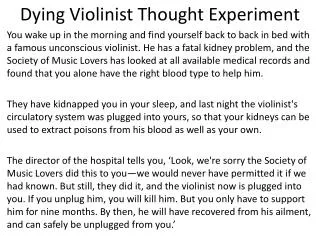
Delayed Reinforcers • Many of life’s reinforcers are delayed… • Eating right, studying, etc. • Delay obviously devalues a reinforcer • How are effects of reinforcers affected by delay? • Why choose the immediate, smaller reward? • Why ever show self-control?
Remember Superstition? • Temporal, not causal • Causal, with delay, very hard • Same with delay of reinforcement • Effects decrease with delay • But how does it occur? • Are there reliable and predictable effects? • Can we quantify the effect?
How Do We Measure Delay Effects? Studying preference of delayed reinforcers Humans: - verbal reports at different points in time - “what if” questions Humans AND nonhumans: A. Concurrent chains B: Titration All are choice techniques. 7
A. Concurrent chains Concurrent chains are simply concurrent schedules -- usually concurrent equal VI VI -- in which reinforcers are delayed. When a response is reinforced, usually both concurrent schedules stop and become unavailable, and a delay starts. Sometimes the delays are in blackout with no response required to get the final reinforcer (an FT schedule); Sometimes the delays are actually schedules, with an associated stimulus, like an FI schedule, that requires responding. 8
Initial links, Choice phase W W Conc VI VI W W W W Terminal links, Outcome phase VI a s VI b s Food Food The concurrent-chain procedure 9
An example of a concurrent-chain experiment MacEwen (1972) investigated choice between two terminal-link FI and two terminal-link VI schedules, one of which was always twice as long as the other. The initial links were always concurrent VI 60-s VI 60-s schedules. 10
The terminal-link schedules were: Constant reinforcer (delay and immediacy) ratio in the terminal links – all immediacy ratios are 2:1. 11
From the generalised matching law, we would expect: If ad was constant, then because D2/D1 was kept constant, we would expect no change in choice with changes in the absolute size of the delays. D2/D1 was kept constant throughout. 13
But choice did change, so ad did NOT remain constant: But does give us some data to answer some other questions… 14
Shape of the Delay Function • Now that we have some data… • How does reinforcer value change over time? • What is the shape of the decay function?
Basically, the effects that reinforcers have on behaviour decrease -- rapidly -- when the reinforcers are more and more delayed after the reinforced response. This is how reinforcer value generally changes with delay: 16
Delay Functions What is the “real” delay function? Vt = V0 / (1 + Kt) Vt = V0/(1 + Kt)s Vt = V0/(M + Kts) Vt = V0/(M + ts) Vt = V0 exp(-Mt)
Exponential versus hyperbolic decay It is important to understand how the effects of reinforcers decay over time, because different sorts of decay predict different effects. The two main candidates: Exponential decay -- the rate of decay remains constant over time in this Hyperbolic decay -- the rate of decay decreases over time -- as in memory, too 18
Exponential decay Vt : value of the delayed reinforcer at time t Vo : value of the reinforcer at 0-s delay t : delay in seconds b : a parameter that determines the rate of decay e : the base of natural logarithms. 20
Hyperbolic decay In this equation, all the variables are the same as in the exponential decay, except that h is the half-life of the decay -- the time over which the value of Vo reduced to half its initial value. Hyperbolic decay is strongly supported by Mazur’s research. 21
Two sorts of decay fitted to McEwen's (1972) data Hyperbolic is clearly better. Not that clean, but… Relative Rate 23
Studying Delay Using Indifference • Titration procedures.
B: Titration - Finding the point of preference reversal The titration procedure was introduced by Mazur: - one standard (constant) delay and - one adjusting delay. These may differ in what schedule they are (e.g., FT versus VT with the same size reinforcers for both), or they may be the same schedule (both FT, say) with different magnitudes of reinforcers. What the procedure does is to find the value of the adjusting delay that is equally preferred to the standard delay -- the indifference point in choice. 25
For example: - reinforcer magnitudes are the same - standard schedule is VT 30 s - adjusting schedule is FT How long would the FT schedule need to become to make preference equal? 26
Titration: Procedure Trials are in blocks of 4. The first 2 are forced choice, randomly one to each alternative The last 2 are free choice. If, on the last 2 trials, it chooses the adjusting schedule twice, the adjusting schedule is increased by a small amount. If it chooses the standard twice, the adjusting schedule is decreased by a small amount. If equal choice (1 of each) -- no change (von Bekesy procedure in audition) 27
Mazur's titration procedure Why the post-reinforcer blackout? ITI W W W Trial start W W W Peck Choice W W W Standard delay + red houselight Adjusting delay + green houselight 2-s food, BO 6-s food 28
Mazur’s Findings • Different magnitudes, finding delay • 2-sec rf delayed 8 sec = 6 sec rf delayed 20 sec. • Equal magnitudes, variable vs. fixed delay • Fixed delay 20 sec = variable delay 30 sec • Why preference for variable? • Hyperbolic decay and interval weighting.
Moving onto Self-Control • Which would you prefer? • $1 in an hour • $2 tomorrow
Moving onto Self-Control • Which would you prefer? • $1 in a month • $2 in a month and a day
Here’s the problem: Preference reversal In positive self control, the further you are away from the smaller and larger reinforcers, the more likely you are to accept the larger, more delayed reinforcers. But, the closer you get to the first one, the more likely you are to chose the smaller, more immediate one. 32
Friday night: “Alright, I am setting my alarm clock to wake me up at 6.00 am tomorrow morning, and then I’ll go jogging.” ... Saturday 6.00 am: “Hmm….maybe not today.” 33
Assume: At the moment in time when we make the choice, we choose the reinforcer that has the highest current value... To be able to understand why preference reversal occurs, we need to know how the value of a reinforcer changes the time by which it is delayed... Outside the laboratory, the majority of reinforcers are delayed. Studying the effects of delayed reinforcers is therefore very important. 35
Animal research: Preference reversal Green, Fisher, Perlow, & Sherman (1981) Choice between a 2-s and a 6-s reinforcer. Larger reinforcer delayed 4 s more than the smaller. Choice response (across conditions) required from 2 to 28 s before the smaller reinforcer. We will call this time T. 36
Large rf Small rf choice 4 s 28 s T 2 s 37
Large rf Small rf choice 4 s 28 s T 2 s 38
Large rf Small rf choice 4 s 28 s T 2 s 39
Green et al. (continued) Thus, if T was 10 s, at the choice point, the smaller reinforcer was 10-s away the larger was 14-s away So, as T is changed over conditions, we should see preference reversal. 40
Control condition: two equal-sized reinforcers were delayed, one 28 s the other 32 s. Preference was strongly towards the reinforcer that came sooner. So, at delays that long, pigeons can still clearly tell which reinforcer is sooner and which one later. Larger, later / Smaller, sooner 41
Hyperbolic predictions shown the same way Choice reverses here 44
Using strict matching theory to explain preference reversal The concatenated strict matching law for reinforcer magnitude and delay (see the generalised matching lecture) is: where M is reinforcer magnitude, and D is reinforcer delay. Note that for delay, a longer delay is less preferred, and therefore D2 is on top. (OK, we know SM isn’t right, and delay sensitivity isn’t constant) 45
We will take the situation used by Green et al. (1981), and work through what the STRICT matching law predicts: The baseline is: M1 = 2, M2 = 6, D1 = 0, D2 = 4 The choice is infinite. Thus, the subject is predicted always to take the smaller, zero-delayed, reinforcer 46
Now, add T = 0.5 s, so M1 = 2, M2 = 6, D1 = 0.5, D2 = 4.5 The subject is predicted to prefer the smaller magnitude reinforcer three times more than the larger magnitude reinforcer, and again be impulsive. But its preference for the immediate reinforcer has decreased a lot. 47
Then, when T = 1, The choice is now less impulsive. 48
For T = 2, the preference ratio B1/B2 is 1 -- so now, the generalised matching law predicts indifference between the two choices. For T = 10, the preference ratio is 0. 47 -- more than 2:1 towards the larger, more delayed, reinforcer. That is, the subject is now showing self control The whole function is shown next -- predictions for Green et al. (1981) assuming strict matching. 49
This graph shows log (B2/B1), rather than (B1/B2), shows how self control increases as you go back in time from when the reinforcers are due. Self control Impulsive 50