Download
1 / 22
220 likes | 339 Vues
This guide provides an overview of R, a programming language and software environment for statistical computing and graphics. Originally developed by Ross Ihaka and Robert Gentleman, R is open-source, free to use, and works on various operating systems including Windows, Mac OS X, and Linux. This introduction covers the R operating environment, basic commands, data import/export, graphic plotting techniques, and example analyses such as T-tests and linear regression. Embrace R for efficient data handling, visualizations, and statistical analyses.

E N D
An Introduction to R Statistical Computing AMS 597
Outline • What’s R? • R Operating Environment • Help and Manuals • Download and install packages • Basic Commands and Functions • Import and Export Data • Graphic Plot • Examples
What’s R? • Programming language and software environment for data manipulation, calculation and graphical display. • Originally created by Ross Ihaka and Robert Gentleman at University of Auckland, and now developed by the R Development Core Team. Where to get R? • http://www.r-project.org/ • Latest Release: R 2.13.0, on April 12, 2011
Why use R? • IT IS FREE • Pre-compiled binary versions are provided for Microsoft Windows, Mac OS X, and several other Linux/Unix-like operating systems • Open source code available freely available on GNU General Public License • For computationally-intensive tasks, C, C++ and Fortran code can be linked and called at run time • An effective data handling and storage facility • A suite of operators for calculations on arrays, in particular matrices • A large, coherent, integrated collection of intermediate tools for data analysis • Graphical facilities for data analysis and display either directly at the computer or on hardcopy
How to Study R • Help Manual • Google!!!
Start with R >help. start() >help(function name) >?function name Example >?lm >??object >help.search(“title”) Example >help.search(“test”) >??colsum
Download and Install Package • All R functions and datasets are stored in packages. Only when a package is loaded, its contents are available. This is down both for efficiency, and to aid package developers. • To see which packages are installed at your site, issue the command • >library(boot) • Users connected to the Internet can use install.packages() and update.packages() to install and update packages. • To see packages currently loaded, use search().
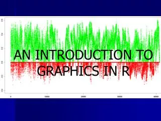
Graphic Plot • Plot Types: Line Charts, Bar Charts, Histograms, Pie Charts, Dot Charts, etc. • Format: >PLOT-TYPE(PLOT-DATA, DETAILS) • PLOT-TYPE: plot, plot.xy, barplot, pie, dotchart, etc. • PLOT-DATA: Data, Data$XXX, as.matrix(Data), etc. • Details: axes, col, pch, lty, ylim, type, xlab, ylab, etc. • For graphics plot: • http://www.harding.edu/fmccown/R/
Example 1: T-test • Generate two datasets X and Y; • Do the Shapiro-Wilk normality test; • Shapiro.test(x) • Do the t-test • Alternative: two sided; less; greater; • Paired or not; • Confidence interval.
Example 1: T-test • t.test(x, y = NULL, alternative = c("two.sided", "less", "greater"), mu = 0, paired = FALSE, var.equal = FALSE, conf.level = 0.95, ...) • Example: t.test(1:10,y=c(7:20)) t.test(1:10,y=c(7:20, 200))
Example 2: Linear Regression • A comparison of GM monthly returns & SP500 monthly returns. GM and SP500 monthly return data during the period of Jan. 2002 to Jun. 2007 are taken. Plotted in R, they will be analyzed and compared. • Data from: http://www.stanford.edu/~xing/statfinbook/data.html
Example 2: Linear Regression GM<-read.table("C:/gm.txt", header=TRUE, sep="") SP<-read.table("C:/sp.txt", header=TRUE, sep="") plot(GM) lines(GM$logret, lty=1) #connect the plots with solid lines lines(SP$logret, type="o", lty=1, pch="+",col="red") #connect with different mark and color x<-1:546 # x here is the time step GML<-lm(GM$logret~x) # linear regression corresponding to time SPL<-lm(SP$logret~x) abline(coef(GML),lwd=3) # abline gives the regression line abline(coef(SPL), col="red", lwd=3) #lwd gives the line width