An Introduction to R graphics
180 likes | 496 Vues
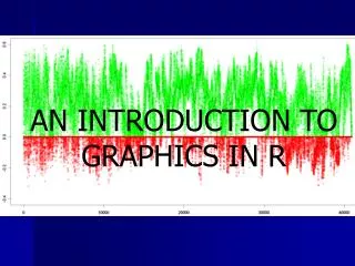
An Introduction to R graphics. Cody Chiuzan Division of Biostatistics and Epidemiology Computing for Research I, 2012. R graphics – Nice and Simple. R has powerful graphics facilities for the production of publication-quality diagrams and plots.

An Introduction to R graphics
E N D
Presentation Transcript
An Introduction to R graphics Cody Chiuzan Division of Biostatistics and Epidemiology Computing for Research I, 2012
R graphics – Nice and Simple R has powerful graphics facilities for the production of publication-quality diagrams and plots. Can produce traditional plots as well as grid graphics. Great reference: Murrell P., R Graphics
Topics for today Histograms Plot, points, lines, legend, xlab, ylab, main, xlim, ylim, pch, lty, lwd. Scatterplot matrix Individual profiles 3D graphs
R code • Data available in R; for a full description: help(Puromycin). • We will start with the basic command plot() and tackle each parameter. • Generate multiple graphs in the same window using: par(mfrow). • For a better understanding use help().
Change parameters using par() A list of graphical parameters that define the default behavior of all plot functions. Just like other R objects, par elements are similarly modifiable, with slightly different syntax. e.g. par(“bg”=“lightcyan”) This would change the background color of all subsequent plots to light cyan When par elements are modified directly (as above, this changes all subsequent plotting behavior.
Par examples modifiable from within plotting functions bg – plot background color lty – line type (e.g. dot, dash, solid) lwd – line width col – color cex – text size inside plot xlab, ylab – axes labels main – title pch – plotting symbol … and many more (learn as you need them)
Great website for choosing colors: http://research.stowers-institute.org/efg/R/Color/Chart/ColorChart.pdf Plotting symbols for pch
Multiple plots • The number of plots on a page, and their placement on the page, can be controlled using par() or layout(). • The number of figure regions can be controlled using mfrow and mfcol. e.g. par(mfrow=c(3,2)) # Creates 6 figures arranged in 3 rows and 2 columns • Layout() allows the creation of multiple figure regions of unequal sizes. e.g. layout(matrix(c(1,2)), heights=c(2,1))
Graph using statistical function output Many statistical functions (regression, cluster analysis) create special objects. These arguments will automatically format graphical output in a specific way. e.g. Produce diagnostic plots from a linear model analysis (see R code) # Reg = lm() # plot(Reg) hclust() agnes() # hierarchical cluster analysis
Save the output • Specify destination of graphics output or simply right click and copy • Could be files • Not Scalable • JPG # not recommended, introduces blurry artifacts around the lines • BMP • PNG • Scalable: • Postscript # preferred in LaTex • Pdf # great for posters
Save the output setwd("") # this is where the plot will be saved pdf(file="Puromycin.pdf“, width = , height = , res = ) dev.off()