Data Display How to Effectively Communicate Your Findings
590 likes | 610 Vues
Learn how to communicate your data effectively in order to draw accurate conclusions, demonstrate professionalism, increase credibility, and better understand your data. Explore various methods such as tables, scatter plots, line graphs, bar charts, histograms, and more. Also, discuss ethical issues in data display and revisit your own work.

Data Display How to Effectively Communicate Your Findings
E N D
Presentation Transcript
Data DisplayHow to Effectively CommunicateYour Findings Mary Purugganan, Ph.D. maryp@rice.edu http://www.owlnet.rice.edu/~cainproj/ Leadership & Professional Development Workshop March 23, 2007
0.0004% 0.05% 0.7% The population of the earth Deevey, E. S., Jr. Scientific American (1960)194–204.
Why improve your data presentation? • To draw accurate conclusions • To demonstrate professionalism • To increase your credibility • To better analyze, synthesize, and understand your data • To see hidden relationships • To appreciate limitations, gaps • To formulate new questions
Today’s plan • Examine function and design • Tables • Scatter plots and line graphs • Bar charts, histograms, frequency polygons • Photographs, micrographs • Diagrams • Video clips • Recognize differences in contexts • Written documents • Visual presentations (posters, oral presentations) • Discuss ethical issues in data display • Revisit your own work
Tables Function • Organize complicated data • Show specific results Known (units) variable/ unknown (units)
Tables Design • Legend • Place above table contents • Must contain table number and title • May contain a caption as well • Avoid rules (gridlines) in small tables • Use rules cautiously in large tables • Choose narrow and/or gray lines • Consider blocks of light color instead of rules
Decked heading Example: Small table Day, R.A. (1998) How to Write and Publish a Scientific Paper. Phoenix: Oryx Press
Example: Rules in large table Rules should be narrow, faint, and unobtrusive J. Donnell, Georgia Tech; http://www.me.vt.edu/writing/handbook
Example: Color bars in large table Color bars aid readers who may have to, for example, look up and compare values often J. Donnell, Georgia Tech; http://www.me.vt.edu/writing/handbook
Bivariate graphs • X/Y axis: independent variable (what you control or choose to observe) vs. dependent variable • Examples: • Scatter plots/ line graphs • Bar graphs/ histograms
Scatterplots and line graphs • Function • Plot two variables; x and y represent actual, continuous space • Good for showing trends / relationships • Design • Avoid legends (keys) off to side in box • Label lines (best for projected work), or • Place key in caption or within graph (written documents)
Scatterplot with key in graph Sanchez et al. (2004) Chem Eng J. 104:1-6
Line graph with key in legend Appropriate for written work, not projection Day, R.A. (1998) How to Write and Publish a Scientific Paper. Phoenix: Oryx Press
Exercise: How would you revise? Balanya et al. Science (2006) 313:1773.
Packed graphs: use with caution Chmiola et al. Science (2006) 313:1760.
Ways to represent data sets Valiela (2001) Doing Science: Design, Analysis, and Communication of Scientific Research. New York: Oxford University Press.
Upper/lower quartiles median Min Ways to represent data sets Max Valiela (2001) Doing Science: Design, Analysis, and Communication of Scientific Research. New York: Oxford University Press.
Bar Graphs Allow comparisons in values when the independent variable is a classification or category Dependent variable Classification or category
Choose the right graph If your variables are categorical (distinct, with no intermediates), you cannot plot with a line graph Nonpoint Source News-Notes 43:5 (1995)
Histograms • Function • Plot frequency vs. intervals of values • Good for seeing shape of the distribution • Good for screening of outliers or checking normality • Not good for seeing exact values (data is grouped into categories) • Design • Bars should touch one another (unlike bar graphs)--lower limit of one interval is also upper limit of previous interval • Use only with continuous data
Example: Histograms Fig. 5. Frequency histograms of ΔP2/μ values using different step distances. At a step distance of 10 μ (a) the percent histogram is symmetric, i.e. positive and negative values have similar frequencies. At larger step distances the histograms become broader (50 μ) and then disintegrate (500 μ). Class size: 1 torr. Baumgartl et al. (2002) Comparative Biochemistry and Physiology 132:75-85.
a, For the coherent splitting, a BEC is produced in the single well, which is then deformed to a double well. We observe a narrow phase distribution for many repetitions of an interference experiment between these two matter waves, showing that there is a deterministic phase evolution during the splitting. b, To produce two independent BECs, the double well is formed while the atomic sample is thermal. Condensation is then achieved by evaporative cooling in the dressed-state potential. The observed relative phase between the two BECs is completely random, as expected for two independent matter waves. S. Hofferberth et al. Radiofrequency-dressed-state potentials for neutral atoms Nature Physics2, - pp710 - 716 (2006)
Exercise: how would you revise these histograms? Fig. 2. (a) Histogram of total detected TPF photons from single-molecule time traces and an exponential fit to the distribution, yielding an e-1 value of 6024 ± 730 photons. A histogram of single-molecule TPF lifetimes of DCDHF-6 in PMMA is shown in (b). The lifetime distribution is fit to a Gaussian; fit parameters are given in the text. Schuck, P.J. et al. (2005) Chemical Physics. 318:7-11.
Frequency Polygons • Function • Constructed from frequency tables • Visually appealing way of showing counts/ frequency • Better than histogram for two sets of data because the graph appears less cluttered • Design • Use a point (instead of histogram bar) and connect the points with straight lines • May shade area underneath the line http://www.olemiss.edu/courses/psy214/Lectures/Lecture2/lex_2.htm
Three-variable graphs • Perspective graphs • Contour plots • See Doing Science: Design, Analysis, and Communication of Scientific Data (Valiela, 2001) Kazhdan, D. et al. (1995) Physics of Fluids 7:2679-2685 http://www.itl.nist.gov/div898/handbook/eda/section3/contour.htm
No chartjunk! Graphical simplicity: keep “data-ink” to “non-data-ink” ratio high 30oC 25oC 20oC Emphasis on data Too much non-data ink
Fill patterns • Avoid moiré effects / vibrations • Gray shading is preferable to hatching • Avoid 3-dimensional bars No chartjunk! • Gridlines • Rarely necessary • Better when thin, gray
Shahbazian et al., Neuron (2002) Photographs • Function • Good for documenting physical observations • Usually qualitative but supported by quantitative data • Design • Place title and caption below photograph(s) • Crop and arrange several photographs to facilitate understanding • Insert scale bars when necessary C.R. Twidale (2004) Earth Sci Rev 67:159-218
Micrographs Fig. 2. GFP.S co-localizes with wild-type S at the ER. Shown is the intracellular distribution of GFP.S expressed either alone (squares a–c) or together with SHA (squares d–i) in COS-7 cells. Cells were fixed, permeabilized, and examined by fluorescence microscopy. (a, d, and g) GFP fluorescence (green); (b and e) immunostaining with a mouse antibody to PDI followed by AlexaFluor 494-conjugated goat anti-mouse IgG (red); (h) immunostaining with a mouse anti-HA antibody followed by AlexaFluor 494-conjugated goat anti-mouse IgG (red) to visualize SHA. Squares c, f, and i are the corresponding merged images so that overlapping red and green signals appear yellow. Fig. 3. STM micrographs of Ag (100). (a) 0.1 Å~0.1 area. (b) Edge enhanced image of (a), (c) 500 ÅÅ~500 Å and (d) 100 ÅÅ~100 Å areas, respectively. Ali et al. (1998) Thin Solid Films 323:105-109 Lambert et al. (2004) Virology 330:158-67
Diagrams & drawings • Function • Show parts and relationships • Focus audience attention to what is essential • Design • Use color to show relationships and draw eye • Avoid unintentional changes in proportion and scale Leuptow, R.M. (June 2004) NASA Tech Briefs.
Video clips • Function • Show processes in real-time • Supplement online journal articles • May be qualitative but supported by quantitative data • Design • No conventions yet observed / published
Video clips Shahbazian et al., (2002) Neuron 35:253-54. Supplemental movie S2 online at: http://www.neuron.org/cgi/content/full/35/2/243/DC1/
Design data display for your context Written documents • Theses • Manuscripts • Reports Visual presentations • Seminars/ oral presentation • Posters
Conventions for written documents • Number and title (caption) each graphic • Table 1. Xxxxxxx… • Figure 3. Xxxxxxx… • Identify graphics correctly • Tables are “tables” • Everything else (graph, illustration, photo, etc.) is a “figure”
Conventions for written documents • Refer to graphics in the text • “Table 5 shows…” • “… as shown in Figure 1.” • “… (Table 2).” • Incorporate graphics correctly • Place graphics close to text reference • Caption correctly • Above tables • Below figures
Tips for written documents • Design graphics for black-and-white printers and photocopies • Figure and table captions can be long and informative (follow individual discipline and journal conventions) • Remember audience when designing • Journals: learn as much as possible about audience to identify needs, areas of expertise • Thesis: design for “outside” committee member
Tips for visual presentations Uniqueness of posters and oral presentations • User is not a reader • Is not able to assimilate great detail • May not have time to process confusing data • Oral communication accompanies what is printed / projected • “Free” and “guaranteed” color • Use color purposefully • Avoid overuse of decorative color • Avoid too much color (e.g., background fill) • Avoid layering two colors of similar intensity (e.g., red on blue) • Be sensitive to red/green color blindness
Visual explanations • Tag image with explanations • Interpret (don’t just show) data (esp. on posters!)
Exercise: How would you revise for PPT? Farchioni et al. Eur. Phys. J. C (2006) 47:461.
Ethics in data display • Putting data in the best light vs. trying to deceive through display • Data can be • Distorted (perceived visual effect different from numerical representation) • Misrepresented (particularly visual data) • Cooked (selecting from among observations) • Mendel? • Trimmed (ignoring extreme values in a data set)
Distortion • Readers do not compare areas in circles correctly (larger circle does not appear to have the increased area it actually does) Number of people on Drug A Number of people on Drug B
Distortion 3-dimensional graphs may fool the eye
most accurateperception least accurateperception Cleveland’s experiments (1985) Accuracy in perceiving graphical cues: Position along axis Length Angle / slope Area Volume Color / shade
How to avoid distortion • Show enough data • Be aware of potential sources of distortion • Scale of graph (limits; log) • Placement of origin • Shape (length of axes) • Omission of data range in a continuum (implied continuum)
Taking a log spreads out small values and compresses larger ones! Linear and logarithmic scales Schulze and Mealy (2001) American Scientist 89: 209.
Ethics in display of visual data Photographic data: Particularly vulnerable to trimming • field of view selection • cropping • software (e.g., Photoshop) manipulation of contrast, brightness, etc. • Editorial in Nature (Feb 23, 2006) • “In Nature’s view, beautification is a form of misrepresentation” • Concise guide to image handling in Guides for Authors (Nature family of journals)
http://www.nature.com/nature/authors/infosheets.html Accessed 10/12/06
Summary • Consider function when choosing visual • Follow design conventions • Adapt visual for context (written vs. visual) • Design for audience • Question your data selection and representation; avoid cooking, trimming, and distortion