Chapter 10 Monopoly
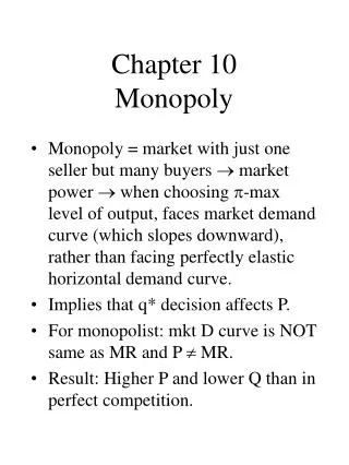
Chapter 10 Monopoly. Monopoly = market with just one seller but many buyers market power when choosing -max level of output, faces market demand curve (which slopes downward), rather than facing perfectly elastic horizontal demand curve. Implies that q* decision affects P.

Chapter 10 Monopoly
E N D
Presentation Transcript
Chapter 10Monopoly • Monopoly = market with just one seller but many buyers market power when choosing -max level of output, faces market demand curve (which slopes downward), rather than facing perfectly elastic horizontal demand curve. • Implies that q* decision affects P. • For monopolist: mkt D curve is NOT same as MR and P MR. • Result: Higher P and lower Q than in perfect competition.
More on Monopoly • When say monopolist faces the market down-sloped D curve: means this firm must consider the market inverse relationship between P and Q; I.e., when Q, must P. • Has implications for AR, MR, and -max q* (which equals Q*). • AR: price per unit sold: this is market demand curve. • MR P since when sell extra Q and P, this P affects ALL Q sold, not just last Q sold.
Monopolist’s -max Decision • AR is market demand curve. • MR lies below AR curve (See Figure 10.1 and Table 10.1.) • Monopolist’s production decisions: • 1) Pick q* where MR = MC. • (This is same rule as in PC except in PC, MR=P.) • 2) Then get P off of D curve. (At q*, how much are buyers willing to pay?) • Note that 0. • See Figure 10.2.
PC vs Monopolist • PC has lower price and higher quantity, has zero profits in LR, and is more efficient (efficiency due to P=MC). • Monopolist has higher price and lower quantity, can have positive profits in LR (due to restricted firm entry), and is less efficient; I.e., imposes a deadweight loss (because PMC). • See Figure 10.3
Pricing for a Monopolist • Eqn. (10.2): P = MC/[1+(1/Ed)] Comes from equation (10.1) showing price mark-up over MC as a % of price. Recall for PC: P = MC. For monopolist: P MC. So HOW much is P greater than MC? Difference depends inversely on Ed. If demand very elasticlittle mark-up, so little benefit to operating as a monopolist. See Figure 10.8. KEY: Monopolist operates only on elastic portion of demand curve.
Price vs MR • Remember two points: • Monopolist operates only on elastic portion of demand curve; • MR P. • MR = P[1+1/ED]. • So if ED -1 then MR 0. In other words: if D is inelastic, then MR is negative. At point that D becomes inelastic, MR curve drops below horizontal axis. So monopolist will not operate on inelastic portion of demand curve.
Examples • 1. Demand not very elastic; So, demand not very responsive to P: Ed = -1.1: • P = MC/[1+(1/Ed)] • P = MC/[1+(1/-1.1)] • P = 10 * MC. • 2. Demand very elastic: • Ed=-5. • P = 1.25 * MC. • Rule: Monopolist gains most when operating on least elastic range (of the elastic portion of D curve).
Other Industry Structures • Some industries don’t have zero market power like PC and not lots of mkt power like monopoly; they lie somewhere in between. • # firms: not huge but not 1. • Product differentiation. • Result: firms don’t face perfectly elastic D curve like in PC but don’t face full market D curve like in monopoly. • See Figure 10.7.
Measuring Market Power • By how much will P exceed MC? • Lerner Index of Monopoly Power: excess of price over MC as fraction of price (from eq.1). • L = (P-MC)/P; 0 L 1. • L = 0 for PC (when P=MC). • Remember: L = -1/ED but now this ED is for a specific firm. • Examples of two groups of buyers: supermarket vs convenience store. • See Figure 10.8.
Sources of Monopoly Power • Factors that affect degree to which a single firm can exert some control over price? • 1) E D power. • 2) # firms power. • -Depends on ease of entry for new firms. • 3) how firms interact: more aggressive competition leads to less market power.
PC vs Monopoly • I. Compare P and Q: PC has lower price and higher Q. • II. Compare PS and CS: Monopoly involves deadweight loss (related to loss in efficiency from non-MC pricing). This deadweight loss is the social cost of monopoly. • See Figure 10.10.
Natural Monopoly • NM occurs in industry in which cost structure differs: now cost advantage to monopoly. • KEY: strong economies of scale so that AC slopes down at all levels of Q. • So MC AC at all Q. • With this cost structure: MORE efficient to operate as NM than PC. • See Figure 10.12.
Exercise • Given that MC = constant = $10 and the following P and Q information,: • Calculate firm’s MR, -max P and Q.
Info for Exercise • Price Quantity27 0 • 24 2 • 21 4 • 18 6 • 15 8 • 12 10 • 9 12 • 6 14 • 3 16 • 0 18

