Download
1 / 32
730 likes | 2.06k Vues
Ch. 3: Inverse Kinematics Ch. 4: Velocity Kinematics. Updates. Labs and section times announced If you haven’t already, please forward your availability to Shelten & Ben Matlab review files are posted. 03_12. Recap: kinematic decoupling. Appropriate for systems that have an arm a wrist

E N D
Ch. 3: Inverse KinematicsCh. 4: Velocity Kinematics ES159/259
Updates • Labs and section times announced • If you haven’t already, please forward your availability to Shelten & Ben • Matlab review files are posted ES159/259
03_12 Recap: kinematic decoupling • Appropriate for systems that have an arm a wrist • Such that the wrist joint axes are aligned at a point • For such systems, we can split the inverse kinematics problem into two parts: • Inverse position kinematics: position of the wrist center • Inverse orientation kinematics: orientation of the wrist • First, assume 6DOF, the last three intersecting at oc • Use the position of the wrist center to determine the first three joint angles… ES159/259
03_12 Recap: kinematic decoupling • Now, origin of tool frame, o6, is a distance d6 translated along z5 (since z5 and z6 are collinear) • Thus, the third column of R is the direction of z6 (w/ respect to the base frame) and we can write: • Rearranging: • Calling o = [oxoyoz]T, oc0 = [xcyczc]T ES159/259
03_12 Recap: kinematic decoupling • Since [xcyczc]T are determined from the first three joint angles, our forward kinematics expression now allows us to solve for the first three joint angles decoupled from the final three. • Thus we now have R30 • Note that: • To solve for the final three joint angles: • Since the last three joints for a spherical wrist, we can use a set of Euler angles to solve for them ES159/259
03_13 Recap: Inverse position kinematics • Now that we have [xcyczc]T we need to find q1, q2, q3 • Solve for qi by projecting onto the xi-1, yi-1 plane, solve trig problem • Two examples • elbow (RRR) manipulator: 4 solutions (left-arm elbow-up, left-arm elbow-down, right-arm elbow-up, right-arm elbow-down) • spherical (RRP) manipulator: 2 solutions (left-arm, right-arm) ES159/259
Inverse orientation kinematics • Now that we can solve for the position of the wrist center (given kinematic decoupling), we can use the desired orientation of the end effector to solve for the last three joint angles • Finding a set of Euler angles corresponding to a desired rotation matrix R • We want the final three joint angles that give the orientation of the tool frame with respect to o3 (i.e. R63) ES159/259
03_03tbl Inverse orientation: spherical wrist • Previously, we said that the forward kinematics of the spherical wrist were identical to a ZYZ Euler angle transformation: ES159/259
03_03tbl Inverse orientation: spherical wrist • The inverse orientation problem reduces to finding a set of Euler angles (q4, q5, q6) that satisfy: • to solve this, take two cases: • Both r13 and r23 are not zero (i.e. q5 ≠ 0)… nonsingular • q5 = 0, thus r13 = r23 = 0… singular • Nonsingular case • If q5 ≠ 0, then r33 ≠ ±1 and: ES159/259
03_03tbl Inverse orientation: spherical wrist • Thus there are two values for q5. Using the first (s5 > 0): • Using the second value for q5 (s5 < 0): • Thus for the nonsingular case, there are two solutions for the inverse orientation kinematics ES159/259
03_03tbl Inverse orientation: spherical wrist • In the singular case, q5 = 0 thus s5 = 0 and r13 = r23 = r31 = r32 = 0 • Therefore, R63 has the form: • So we can find the sum q4 + q6 as follows: • Since we can only find the sum, there is an infinite number of solutions (singular configuration) ES159/259
Inverse Kinematics: general procedure • Find q1, q2, q3 such that the position of the wrist center is: • Using q1, q2, q3, determine R30 • Find Euler angles corresponding to the rotation matrix: inverse position kinematics inverse orientation kinematics ES159/259
03_22 Example: RRR arm with spherical wrist • For the DH parameters below, we can derive R30 from the forward kinematics: • We know that R63 is given as follows: • To solve the inverse orientation kinematics: • For a given desired R ES159/259
03_22 Example: RRR arm with spherical wrist • Euler angle solutions can be applied. Taking the third column of (R30)TR • Again, if q5 ≠ 0, we can solve for q5: • Finally, we can solve for the two remaining angles as follows: • For the singular configuration (q5 = 0), we can only find q4 + q6 thus it is common to arbitrarily set q4 and solve for q6 ES159/259
03_22 Example: elbow manipulator with spherical wrist • Derive complete inverse kinematics solution • we are given H = T60 such that: ES159/259
03_22 Example: elbow manipulator with spherical wrist • First, we find the wrist center: • Inverse position kinematics: • Where d is the shoulder offset (if any) and D is given by: ES159/259
03_22 Example: elbow manipulator with spherical wrist • Inverse orientation kinematics: • Now that we know q1, q2, q3, we know R30. need to find R36: • Solve for q4, q5, q6, Euler angles: ES159/259
03_22 Example: inverse kinematics of SCARA manipulator • We are given T40: ES159/259
03_22 Example: inverse kinematics of SCARA manipulator • Thus, given the form of T40, R must have the following form: • Where a is defined as: • To solve for q1 and q2 we project the manipulator onto the x0-y0 plane: • This gives two solutions for q2: • Once q2 is known, we can solve for q1: • q4 is now give as: • Finally, it is trivial to see that d3 = oz + d4 ES159/259
03_22 Example: number of solutions • How many solutions to the inverse position kinematics of a planar 3-link arm? • given a desired d=[dxdy]T, the forward kinematics can be written as: • Therefore the inverse kinematics problem is under-constrained (two equations and three unknowns) ∞ solutions is d is inside the workspace 1 solution if d is on the workspace boundary 0 solutions else ES159/259
03_22 Example: number of solutions • What if now we describe the desired position and orientation of the end effector? • given a desired d=[dxdy]T, we can now call the position of o2 the ‘wrist center’. This position is given as: • Now we have reduced the problem to finding the joint angles that will give the desired position of the wrist center (we have done this for a 2D planar manipulator). • Finally, q3 is given as: ∞ solutions if the wrist center is on the origin 2 solutions if wrist center is inside the 2-link workspace 1 solution if wrist center is on the 2-link workspace boundary 0 solutions else ES159/259
Inverse kinematics: more general procedures • Paden-Kahan subproblems • An attempt to create a generalized formulation for solving inverse kinematics based (again) upon some common configurations • This typically involves rotating vectors about moving axes and projecting the rotations onto orthogonal planes to solve for rotation angles • See Murray, Li, Sastry, pp. 99-107 ES159/259
Velocity Kinematics • Now we know how to relate the end-effector position and orientation to the joint variables • Now we want to relate end-effector linear and angular velocities with the joint velocities • First we will discuss angular velocities about a fixed axis • Second we discuss angular velocities about arbitrary (moving) axes • We will then introduce the Jacobian • Instantaneous transformation between a vector in Rn representing joint velocities to a vector in R6 representing the linear and angular velocities of the end-effector • Finally, we use the Jacobian to discuss numerous aspects of manipulators: • Singular configurations • Dynamics • Joint/end-effector forces and torques ES159/259
Angular velocity: fixed axis • When a rigid body rotates about a fixed axis, every point moves in a circle • Let k represent the fixed axis of rotation, then the angular velocity is: • The velocity of any point on a rigid body due to this angular velocity is: • Where r is the vector from the axis of rotation to the point • When a rigid body translates, all points attached to the body have the same velocity ES159/259
Angular velocity: arbitrary axis • Skew-symmetric matrices • Definition: a matrix S is skew symmetric if: • i.e. • Let the elements of S be denoted sij, then by definition: • Thus there are only three independent entries in a skew symmetric matrix • Now we can use S as an operator for a vector a = [axayaz]T ES159/259
Angular velocity: arbitrary axis • Example: • Let i, j, k be defined as follows: • Then we can define the skew symmetric matrices S(i), S(j), S(k): ES159/259
Angular velocity: arbitrary axis • Properties of skew-symmetric matrices • The operator S is linear • The operator S is known as the cross product operator • This can be seen by the definition of the cross product: ES159/259
Angular velocity: arbitrary axis • Properties of skew-symmetric matrices • For • This can be shown for and R as follows: • This can be shown by direct calculation. Finally: • For any ES159/259
Angular velocity: arbitrary axis • Derivative of a rotation matrix • let R be an arbitrary rotation matrix which is a function of a single variable q • R(q)R(q)T=I • Differentiating both sides (w/ respect to q) gives: • Now define the matrix S as: • Then ST is: • Therefore S + ST = 0 and ES159/259
Angular velocity: arbitrary axis • Example: let R=Rx,q, then using the previous results we have: ES159/259
Angular velocity: arbitrary axis • Now consider that we have an angular velocity about an arbitrary axis • Further, let R = R(t) • Now the time derivative of R is: • Where w(t) is the angular velocity of the rotating frame ES159/259
Next class… • Derivation of the Jacobian ES159/259