Download
1 / 12
120 likes | 147 Vues
Explore short-run production, costs, supply curve, factors' optimization, and market dynamics. Learn through examples like Nissan's UK plant decision. Understand production functions, diminishing marginal returns, and product curve relationship.

E N D
Introduction to Microeconomics (L11100) Lectures 12 - 18 Section Four: The Firm’s Supply
Section Outline 4.1 Short Run Production (Lecture 12) 4.2 Short Run Costs (Lecture 13) 4.3 Short Run Supply Curve (Lecture 14) 4.4 Long Run Production (Lecture 15) 4.5 Optimisation of Factor Use and Long- run Costs (Lecture 16) 4.6 Markets (Lecture 17)
4.1 Short Run Production 4.1.1 Production Defined 4.1.2 The Relationship between Output and Inputs 4.1.3 Production in Diagrams
Application “Why Nissan Chose to Stay in the UK” BBC website 24th September 2004 • Nissan decide to produce its people carrier (the Tone) in Sunderland despite threats to go to mainland Europe • Labour costs and working hours mattered • "If you look at the figures.. it makes more sense to build on your existing base because you have existing investments, you have less fixed costs and you have more flexibility than if you develop a new plant from scratch.” Louis Schweitzer, chief executive of Renault. • Scenic – added a third shift • "Which meant no investment, no fixed costs, no extra white collars - only extra blue collars, and 50% additional capacity, which for two lines producing 60 cars per hour is equivalent to a (new) plant” (ditto)
4.1.1 Defining Production Simple description: Inputs are combined to produce outputs Combination is called a PRODUCTION FUNCTION, a general form example of which is: Q = f (land, labour, capital, entrepreneur etc)
Short Run - most factors are fixed, one varies Long Run - all factors vary, technology is unchanged Very Long Run - technology changes as well CETERIS PARIBUS (“all other things equal”) in short run:
4.1.2 The Relationship betweenOutput and Inputs An orchard owner produces apples. Without labour, output is zero. Workers are then hired. Worker Boxes of Apples 1 10 22 2 3 29 4 33 30 5
Q 33 X 29 X X 22 X 10 X L 3 4 5 1 2
Illustrates the LAW OF DIMINISHING MARGINAL RETURNS (Important - short run only) “When successive increases in a variable factor are added to a fixedquantity of another factor the resulting additions to output will eventually fall” Same for all variable factors, not just labour e.g. fertilisers
4.1.3 Production in Diagrams Let us now call total output TOTAL PRODUCT or Average Product: output per worker or TP/L Marginal Product: addition to output from last worker employed
Q TP L Q1 Q2 Q3 Q MP AP L Q1 Q2
Shape of these curves determined by the Law of Diminishing Marginal Returns However, positionis set by level of fixed input Interim Summary 1. Production shows the relationship between inputs and outputs 2. Articulated via the production function 3. In the short run the Law of Diminishing Marginal Returns determines the shape of product curves (TP, AP, MP)