Download
1 / 48
490 likes | 659 Vues
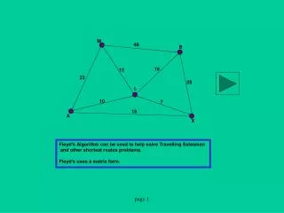
M. 48. B. 19. 10. 23. 20. L. 10. 7. 18. A. X. Floyd’s Algorithm can be used to help solve Travelling Salesman and other shortest routes problems. Floyd’s uses a matrix form. To look back at the network click here:. D( 0 ). R( 0 ). This is the route matrix.

E N D
M 48 B 19 10 23 20 L 10 7 18 A X Floyd’s Algorithm can be used to help solve Travelling Salesman and other shortest routes problems. Floyd’s uses a matrix form. page 1
To look back at the network click here: D( 0 ) R( 0 ) This is the route matrix. It will eventually show the next vertex that needs to be taken on route to finding the shortest route to another vertex. This is the distance matrix. It initially shows the direct distance between one vertex and the others. The infinity sign denotes no direct route. • To view the process step by step click here • To view the completed matrices click here page 2
We highlight the first column and row of the Distance matrix and compare all other items with the sum of the items highlighted in the same row and column. If the sum is less than the item then it should be replaced with the sum. D( 0 ) R( 0 ) Click here to see step:
We highlight the first column and row of the Distance matrix and compare all other items with the sum of the items highlighted in the same row and column. If the sum is less than the item then it should be replaced with the sum. D( 0 ) R( 0 ) 23 + 23 = 46, less than so change. Click here to see step:
We highlight the first column and row of the Distance matrix and compare all other items with the sum of the items highlighted in the same row and column. If the sum is less than the item then it should be replaced with the sum. D( 0 ) R( 0 ) 23 + 23 = 46, less than so change. Click here to see step:
We highlight the first column and row of the Distance matrix and compare all other items with the sum of the items highlighted in the same row and column. If the sum is less than the item then it should be replaced with the sum. D( 0 ) R( 0 ) 10 + 23 = 33, so we leave this item Click here to see step:
We highlight the first column and row of the Distance matrix and compare all other items with the sum of the items highlighted in the same row and column. If the sum is less than the item then it should be replaced with the sum. D( 0 ) R( 0 ) When is involved we leave the item. Click here to see step:
We highlight the first column and row of the Distance matrix and compare all other items with the sum of the items highlighted in the same row and column. If the sum is less than the item then it should be replaced with the sum. D( 0 ) R( 0 ) 18 + 23 = 41, so we replace the item. Click here to see step:
We highlight the first column and row of the Distance matrix and compare all other items with the sum of the items highlighted in the same row and column. If the sum is less than the item then it should be replaced with the sum. D( 0 ) R( 0 ) 18 + 23 = 41, so we replace the item. Click here to see step:
We highlight the first column and row of the Distance matrix and compare all other items with the sum of the items highlighted in the same row and column. If the sum is less than the item then it should be replaced with the sum. D( 0 ) R( 0 ) 23 + 10 = 33, so we leave this item. Click here to see step:
We highlight the first column and row of the Distance matrix and compare all other items with the sum of the items highlighted in the same row and column. If the sum is less than the item then it should be replaced with the sum. D( 0 ) R( 0 ) 10 + 10 = 20, so we replace this item. Click here to see step:
We highlight the first column and row of the Distance matrix and compare all other items with the sum of the items highlighted in the same row and column. If the sum is less than the item then it should be replaced with the sum. D( 0 ) R( 0 ) Infinity is involved so we leave this item. Click here to see step:
We highlight the first column and row of the Distance matrix and compare all other items with the sum of the items highlighted in the same row and column. If the sum is less than the item then it should be replaced with the sum. D( 0 ) R( 0 ) 18 + 10 = 28 which is more than 7 so we leave this item. Click here to see step:
We highlight the first column and row of the Distance matrix and compare all other items with the sum of the items highlighted in the same row and column. If the sum is less than the item then it should be replaced with the sum. D( 0 ) R( 0 ) Infinity is involved so we leave this item. Click here to see step:
We highlight the first column and row of the Distance matrix and compare all other items with the sum of the items highlighted in the same row and column. If the sum is less than the item then it should be replaced with the sum. D( 0 ) R( 0 ) Infinity is involved so we leave this item. Click here to see step:
We highlight the first column and row of the Distance matrix and compare all other items with the sum of the items highlighted in the same row and column. If the sum is less than the item then it should be replaced with the sum. D( 0 ) R( 0 ) Infinity is involved so we leave this item. Click here to see step:
We highlight the first column and row of the Distance matrix and compare all other items with the sum of the items highlighted in the same row and column. If the sum is less than the item then it should be replaced with the sum. D( 0 ) R( 0 ) Infinity is involved so we leave this item. Click here to see step:
We highlight the first column and row of the Distance matrix and compare all other items with the sum of the items highlighted in the same row and column. If the sum is less than the item then it should be replaced with the sum. D( 0 ) R( 0 ) We replace this item with 23 + 18 = 41 Click here to see step:
We highlight the first column and row of the Distance matrix and compare all other items with the sum of the items highlighted in the same row and column. If the sum is less than the item then it should be replaced with the sum. D( 0 ) R( 0 ) We replace this item with 23 + 18 = 41 Click here to see step:
We highlight the first column and row of the Distance matrix and compare all other items with the sum of the items highlighted in the same row and column. If the sum is less than the item then it should be replaced with the sum. D( 0 ) R( 0 ) 10 + 18 = 28, 7 is less than this so leave it. Click here to see step:
We highlight the first column and row of the Distance matrix and compare all other items with the sum of the items highlighted in the same row and column. If the sum is less than the item then it should be replaced with the sum. D( 0 ) R( 0 ) Infinity is involved so leave this item. Click here to see step:
We highlight the first column and row of the Distance matrix and compare all other items with the sum of the items highlighted in the same row and column. If the sum is less than the item then it should be replaced with the sum. D( 0 ) R( 0 ) 18 + 18 = 36, so replace this item. Click here to see step:
We highlight the first column and row of the Distance matrix and compare all other items with the sum of the items highlighted in the same row and column. If the sum is less than the item then it should be replaced with the sum. D( 0 ) R( 0 ) 18 + 18 = 36, so replace this item. Click here to see step:
D( 0 ) R( 0 ) Click here to see step:
D( 0 ) R( 0 ) Click here to see step:
D( 0 ) R( 0 ) Click here to see step:
D( 0 ) R( 0 ) Click here to see step:
D( 0 ) R( 0 ) Click here to see step:
D( 0 ) R( 0 ) Click here to see step:
We have now completed one iteration. We rename the new matrices: D( 1 ) R( 1 ) Subsequent iterations are now shown completed: Click here to see step: Click here to see final matrices:
D( 1 ) R( 1 ) Subsequent iterations are now shown completed: Click here to see step: Click here to see final matrices:
The items have been altered accordingly: D( 1 ) R( 1 ) Subsequent iterations are now shown completed: Click here to see step: Click here to see final matrices:
We can now rename the matrices: D( 2 ) R( 2 ) Click here to see step: Click here to see final matrices:
Next iteration: D( 2 ) R( 2 ) Click here to see step: Click here to see final matrices:
Next iteration, the items are altered appropriately : D( 2 ) R( 2 ) Click here to see step: Click here to see final matrices:
The matrices are renamed : D( 3 ) R( 3 ) Click here to see step: Click here to see final matrices:
The next iteration : D( 3 ) R( 3 ) Click here to see step: Click here to see final matrices:
In this iteration, you do not need to change any of the items, so we go onto the next iteration : D( 3 ) R( 3 ) Click here to see step: Click here to see final matrices:
D( 4 ) R( 4 ) Click here to see step: Click here to see final matrices:
There is only one item that we need to change in this case: D( 4 ) R( 4 ) Click here to see step: Click here to see final matrices:
These are the final matrices, remember that you can use them to redraw the original network. You can then use this to help us solve travelling salesman problems: D( 5 ) R( 5 ) Click here to see new network:
29 17 M 29 B 19 10 20 20 L 10 7 17 A X This network now gives you a better idea of the quickest routes. Click below to try a question: The route matrix gives us an idea about the next vertex to visit on route - 1 represents A, 2 - M, etc. page 1
1 5 4 3 2 15 32 30 35 75 70 40 Try this one! Click below when you have completed it to check the answers:
These are the completed matrices. Are yours correct? D( 5 ) R( 5 )
1 5 4 3 2 Qu2. 35 50 15 12 20 10 50 Answers…………….
These are the completed matrices. Are yours correct? D( 5 ) R( 5 )
1 4 3 2 Qu2. 3 5 3 8 2 4 Answers…………….
These are the completed matrices. Are yours correct? D( 4 ) R( 4 )