Download
1 / 13
130 likes | 215 Vues
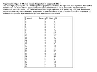
Supplemental Figure 1. Different modes of regulation in response to CN.

E N D
Supplemental Figure 1. Different modes of regulation in response to CN. The following 9 pages (Figures 1A, 1B and 1C) contain graphs that summarize the expression level of genes in the C and/or N treatments. The X-axis in these graphs correspond to the treatment carried out as described in the manuscrpt and summarized in the table below . The Y-axis represents the average expression of all genes (Log2 scale) with the indicated regulatory pattern (e.g. +N-independent). The number “n” of genes classified in each pattern is indicated in parenthesis. (A) N-independent patterns (B) C-independent patterns (C) CN interaction patterns. Treatment Sucrose (mM) Nitrate (mM) 1 30 0 2 30 0 3 60 0 4 60 0 5 90 0 6 90 0 7 30 5 8 60 10 9 90 15 10 30 1.7 11 60 3.3 12 90 5 13 30 15 14 60 30 15 90 45 16 30 5 17 60 10 18 90 15 19 30 1.7 20 60 3.3 21 90 5 22 30 15 23 60 30 24 90 45 25 0 5 26 0 5 27 0 10 28 0 10 29 0 15 30 0 15
-N independent (n=445) 2 1 - - - - - - - - - - - - Mean( log2(ratio) ) 0 - - - - - - - - - - - - - - - - - - - - - - - - - - - - - - - - - - - - - - - - - - - - - - - - +N independent (n=319) -1 2 -2 1 - - - - - - - - - - - 0 5 10 - 15 20 25 30 - - - - - - - - - - - - - - - - - - - - - - - - - - - - - - - - - - - - Mean( log2(ratio) ) 0 Treatments - - - - - - - - - - - - -1 -2 0 5 10 15 20 25 30 Treatments Supplemental figure 1AModel 1 (N-independent)
+C independent (n=1104) 2 1 - - - - - - - - - - - - - - - - - - - - - - - - - - - - - - - - - - - - - - - - - - - - - - - - - - Mean( log2(ratio) ) - - - - - - 0 - - - - -1 -2 0 5 10 15 20 25 30 Treatments -C independent (n=1461) 2 1 - - - Mean( log2(ratio) ) - 0 - - - - - - - - - - - - - - - - - - - - - - - - - - - - - - - - - - - - - - - - - - - - - - - - - - - - - - - - -1 -2 0 5 10 15 20 25 30 Treatments Supplemental figure 1BModel 2 (C-independent)
+C CN N (n=331) 2 - 1 - - - - - - - - - - - - - - - - - - - - - - - - - - - - - - - - - - - - - - - - - - - - - - - - - - - Mean( log2(ratio) ) -C CN N (n=157) - - 0 - - - - - - 2 -1 1 -2 - - - - - Mean( log2(ratio) ) - - - - - - 0 - - - - - - - - - - - - - - - - - - - - - - - - - 0 5 10 15 20 25 30 - - - - - - - - - - - - - - - - - - - - - Treatments - - -1 - -2 0 5 10 15 20 25 30 Treatments Supplemental figure 1CModel 3 ( CN interactions )* *: Patterns with less than 10 genes are not shown.
-C -CN -N (n=103) 2 1 Mean( log2(ratio) ) 0 - - - - - - - - - - - - - - - - - - - - - - - - - - - - - - - - -1 - - - - - - - - - - - - - - - - - - - - - - - - - - - - -2 0 5 10 15 20 25 30 Treatments C CN +N (n=76) C +CN N (n=152) C –CN N (n=81) 2 2 2 - - 1 1 1 - - - - - - - - - - - - - - - - - - - - - - - - - - - - - - - - - - - - - - - - - - - - - - - - - - - - - - - - - - - - - - - - - - - - - - - - - - - - - - - - - - - - Mean( log2(ratio) ) Mean( log2(ratio) ) Mean( log2(ratio) ) - - - - - - - - - - - 0 - 0 0 - - - - - - - - - - - - - - - - - - - - - - - - - - - - - - - - - - - - - - - - - - - - - - - - - - - - - - - - - - - - - - - - - - - - - - - - - - - - - - - - - - -1 -1 -1 -2 -2 -2 0 0 5 5 10 10 15 15 20 20 25 25 30 30 0 5 10 15 20 25 30 Treatments Treatments Treatments Supplemental figure 1C – Cont.
C CN -N (n=49) 2 1 - - - - - - - - - - - - - Mean( log2(ratio) ) - - - 0 - - - - - - - - - - - - - - - - - - - - - - - - - - - - - - - - - - - - - - - - - - - - -1 -2 0 5 10 15 20 25 30 Treatments -C CN -N (n=71) +C CN +N (n=33) --C -CN N (n=40) 2 2 2 1 1 1 - - - - - - - - - - - - - - - - - - - - - - - - - - - - - - - - - - - - - - - - - - - - - - - - - - - Mean( log2(ratio) ) Mean( log2(ratio) ) Mean( log2(ratio) ) - - - - 0 0 0 - - - - - - - - - - - - - - - - - - - - - - - - - - - - - - - - - - - - - - - - - - - - - - - - - - - - - - - - - - - - - - - - - - - - - - - - - - - - - - - - - - - - - - - - - - - - - - - - - - - - - - - - - - - - - - - - - - - - - - -1 -1 -1 - - - - - - - -2 -2 -2 0 0 0 5 5 5 10 10 10 15 15 15 20 20 20 25 25 25 30 30 30 Treatments Treatments Treatments Supplemental figure 1C – Cont.
C -CN +N (n=17) +C -CN N (n=16) ++C +CN N (n=28) C ++CN +N (n=20) 2 2 2 2 - - - - - - - - - - - - - - - - - - - - - - - - - - - - - - - - - - - - - - - - - - - 1 1 1 1 - - - - - - - - - - - - - - - - - - - - - - - - - - - - - - - - - - - - - - - - - - - - - - - - - - - - - - - - - - - - - - - - - - - - - - - - - - - - - - - - - - - - - - - - - - - - - - - - Mean( log2(ratio) ) Mean( log2(ratio) ) - Mean( log2(ratio) ) Mean( log2(ratio) ) - 0 0 0 0 - - - - - - - - - - - - - - - - - - - - - - - - - - - - - - - - - - - - - - - - - - - - - - - - - - - - - - - - - - - - - - - - - - - - - - - - - - - - - - - - - - - - - - - - - - - - - - - -1 -1 -1 -1 - - - - -2 -2 -2 -2 0 0 5 5 10 10 15 15 20 20 25 25 30 30 0 0 5 5 10 10 15 15 20 20 25 25 30 30 Treatments Treatments Treatments Treatments Supplemental figure 1C – Cont.
++C +CN +N(n=15) 2 1 - - - - - - - - - - - - - - - - - - - - - - - - - - - - - - - - - - - - - - - - - - - - - - - - - - - - - - - - - - - - Mean( log2(ratio) ) 0 -1 -2 0 5 10 15 20 25 30 Treatments Supplemental figure 1C – Cont.
+C -N (n=60) 2 - - - - 1 - - - - - - - - - - - - - - - - - - - - - - - - - - - - - - - - - - - - - - - - - - - Mean( log2(ratio) ) - 0 - - - - - - - - - - - - -1 -2 0 5 10 15 20 25 30 Treatments Supplemental figure 1C – Cont. Model 3 (additiveCN interactions) +C +N (n=172) 2 - - - - - - - - - 1 - - - - - - - - - - - - - - - - - - - - - - - - - - - - - - - - - - - - - - - - - - - - - - - - - Mean( log2(ratio) ) - - 0 -1 -2 0 5 10 15 20 25 30 Treatments -C -N (n=136) -C +N (n=98) 2 2 1 1 - - - - - - - - - - - - Mean( log2(ratio) ) Mean( log2(ratio) ) 0 - - 0 - - - - - - - - - - - - - - - - - - - - - - - - - - - - - - - - - - - - - - - - - - - - - - - - - - - - - - - - - - - - - - - - - - - - - - - - - - - - - - - - - - - - - - - - - - - - - - - - - -1 -1 - - - - - - - - - -2 -2 0 5 10 15 20 25 30 0 5 10 15 20 25 30 Treatments Treatments
Supplemental figure 2 A B NO3 assimilation A. thaliana metabolic & regulatory network
Supplemental Figure 2. Construction of a qualitative network model of the plant cell (A)A “bird-eye’s” view of the integrated gene network model. We collected information for Arabidopsis metabolic pathways from the KEGG (1) and AraCyc (2) databases. In addition, we obtained known protein:protein interactions and protein:DNA interactions from Transfac (3), DIP (4) and BIND (5) databases. We used the predicted protein:DNA interactions available from AGRIS (6), the interolog and regulogs described previously (7). In addition, we used experimentally determined protein:protein interactions for D. melanogaster, S. cerevisiae, and C. elegans available from DIP and BIND to infer protein:protein interactions in Arabidopsis. Two Arabidopsis proteins were predicted to interact when the corresponding homologs were known to interact in worm, fly or yeast. For homology we used the NCBI database Homologene (http://www.ncbi.nlm.nih.gov/entrez/query.fcgi?db=homologene). All the interaction data (metabolic, physical, regulatory, etc.) was represented as a qualitative network graph. Genes and metabolites were represented as labeled nodes, and associations between them were represented as labeled edges. Color and shapes were assigned to differentiate types of nodes (e.g. genes, RNA, metabolites) and edges (e.g. enzymatic reaction, transport). The network graph used in this manuscript and a description for each type of label are available in Additional data files 3 and 4 respectively, and also from our accompanying website (http://www.virtualplant.org). We used the open-source Cytoscape software (8) to visualize and query the molecular network for attributes of interest. We used this integrated network representation of the available data as a scaffold on which to analyze the expression data. Because all connections in the network are labeled, the evidence connecting any two nodes or sub-regions in the network can be readily evaluated. All data files were manipulated with custom PERL scripts and stored in a local database. (B) A close-up view of the genes and metabolites involved in the NO3- reduction and assimilation pathway. Zoom into the NO3- reduction pathway. Yellow circles represent metabolites. Blue hexagons represent genes coding for transporters or enzymes. From top to bottom: extracellular NO3- is connected by a blue dotted edge to several genes coding for known or putative transporters. The transporters are in turn connected to intracellular NO3-. Intracellular NO3- is converted to NO2- by the action of nitrate reductase, for which there are two genes in Arabidopsis. NO2- is then reduced to NH3 by the single gene enzyme nitrite reductase. NH3 is subsequently assimilated into amino acids by the GS/GOGAT cycle (not shown). Black and grey edges denote association through enzymatic reactions. Black edges indicate “important” metabolites (shown in the KEGG metabolic pathways). Other interactions (e.g. protein:DNA and protein:protein) are also color-coded but are not shown in this panel. References 1.Kanehisa, M., Goto, S., Kawashima, S. & Nakaya, A. (2002) Nucleic Acids Research30, 42-46. 2.Mueller, L. A., Zhang, P. & Rhee, S. Y. (2003) Plant Physiol132, 453. 3.Matys, V., Fricke, E., Geffers, R., GoSzling, E., Haubrock, M., Hehl, R., Hornischer, K., Karas, D., Kel, A. E. & Kel-Margoulis, O. V. (2003) Nucleic Acids Res31, 374 - 378. 4.Xenarios, I., Salwinski, L., Duan, X. J., Higney, P., Kim, S. M. & Eisenberg, D. (2002) Nucleic Acids Res30, 303-5. 5.Alfarano, C., Andrade, C. E., Anthony, K., Bahroos, N., Bajec, M., Bantoft, K., Betel, D., Bobechko, B., Boutilier, K., Burgess, E., et al. (2005) Nucl. Acids Res.33, D418-424. 6.Davuluri, R., Sun, H., Palaniswamy, S., Matthews, N., Molina, C., Kurtz, M. & Grotewold, E. (2003) BMC Bioinformatics4, 25. 7.Yu, H., Luscombe, N. M., Lu, H. X., Zhu, X., Xia, Y., Han, J. D., Bertin, N., Chung, S., Vidal, M. & Gerstein, M. (2004) Genome Res14, 1107-18. 8.Shannon, P., Markiel, A., Ozier, O., Baliga, N. S., Wang, J. T., Ramage, D., Amin, N., Schwikowski, B. & Ideker, T. (2003) Genome Res.13, 2498-2504.
+C -C +N -N CN interaction Supplemental figure 3
Supplemental figure 4. Comparison of microarray and Q-PCR data. The expression levels determined by Q-PCR data, 8h after CN treatment for TIR1, two auxin-response factors and two auxin efflux carriers is compared to the data obtained in the microarray experiments. Y-axis, mean +/- standard error of the mean. Microarray data n=18. Q-PCR data n≥5. “*” indicates statistically significant repression in the Q-PCR experiments as determined by t-test (p-value ≤ 0.05). All genes showed statistically significant repression in the microarray experiments. At1g59750 At2g17500 At1g76520 At5g62000 At3g62980 0 -0.5 -1 * -1.5 Fold repression log2(Treatment/Control) Microarray * Q-PCR -2 -2.5 * -3 * -3.5